1 Kidney Function and Mortality in the United Arab Emirates - A Predictive Modeling Approach: Python Code
by Leonid Shpaner
This notebook delves into the intricate landscape of kidney function and mortality using Python. Through data exploration, visualization, and machine learning techniques, it aims to provide insights into the prevalence, risk factors, and predictive modeling of mortality with respect to kidney failure in the UAE.
The burden of Chronic Kidney Disease (CKD) is a pressing global health issue, and its impact on public health in the UAE is of particular concern. By leveraging Python's powerful libraries such as Pandas, NumPy, Matplotlib, and scikit-learn, a robust analytical framework has been developed to tackle this challenge head-on.
Throughout this notebook, you'll find detailed explanations, code snippets, visualizations, and interpretations of the data. The analysis aims to maintain clarity and transparency, making it accessible to both technical and non-technical audiences alike.
Whether you're a healthcare professional, data scientist, or simply curious, this notebook serves as a valuable resource for exploring, analyzing, and contributing to furthering our understanding of Chronic Kidney Disease in the United Arab Emirates.
Let's dive into the code and uncover the insights together!
from google.colab import drive
drive.mount("/content/drive") # Mount Google Drive

import sys # Add virtual env's site-packages to sys.path
sys.path.append('/content/drive/MyDrive/ckd_env/lib/python3.10/site-packages')

# Change working directory
%cd '/content/drive/MyDrive/kidney_uae/'

# Prepare activation script for virtual env
!echo "source /content/drive/MyDrive/ckd_env/bin/activate" > activate.sh

# Make scripts and binaries executable
!chmod +x activate.sh
!chmod +x /content/drive/MyDrive/ckd_env/bin/python
!chmod +x /content/drive/MyDrive/ckd_env/bin/pip

%env BASH_ENV=activate.sh # Set BASH_ENV to activate virtual env

print() # New line for clarity
!python --version # Check Python version
2 Preprocessing: Kidney_UAE
2.1 Load Requisite Libraries
######################## Standard Library Imports ##############################
import pandas as pd
import numpy as np
from itertools import combinations
import matplotlib.pyplot as plt
import seaborn as sns
import os
import subprocess

##################### import model libraries ###################################
from sklearn.linear_model import LogisticRegression
from sklearn.svm import SVC
from sklearn.ensemble import RandomForestClassifier, ExtraTreesClassifier
from sklearn.pipeline import Pipeline
from sklearn.model_selection import GridSearchCV, train_test_split
from sklearn.preprocessing import StandardScaler
from sklearn.tree import plot_tree
from sklearn.calibration import calibration_curve, CalibratedClassifierCV
from lifelines import CoxPHFitter, KaplanMeierFitter
import shap  # shap explainer library
################################################################################

######################### import model metrics #################################
from sklearn.metrics import (
    roc_curve,
    auc,
    precision_score,
    recall_score,
    average_precision_score,
    precision_recall_curve,
    r2_score,
    brier_score_loss,
    confusion_matrix,
)

########################### Miscellaneous ######################################
from tqdm import tqdm
import warnings
warnings.filterwarnings("ignore") # suppress warnings

from functions import *  # import custom functions
################################################################################
##################### import Bias & Fairness Analysis Tools ####################
from aequitas import Audit
################################################################################
2.2 Read File From Path and Explore Basic Structure
# Change directory to where functions.py is located if it's not in '/content'
data_path = "/content/drive/MyDrive/kidney_uae/data/"
eda_path = "/content/drive/MyDrive/kidney_uae/data/df_eda/"
image_path = "/content/drive/MyDrive/kidney_uae/images/"
# read in the data from an excel file
df = pd.read_excel(os.path.join(data_path, "kidney_uae.xlsx")).set_index("id")
print(f"There are {df.shape[0]} rows and {df.shape[1]} columns in this dataset.")
df.head() # print first 5 rows of dataframe
2.3 Reorder and Rename Columns
# Shift column 'time(months)' one place to the left
df = move_column_before(
    df=df,
    target_column="time(months)",
    before_column="sex",
)
print(f"New order of columns: {df.columns.to_list()}") # list new order of cols
# rename the following colnames: time(months), creatnine
df.rename(
    columns={"time(months)": "time_months", "creatnine": "creatinine"},
    inplace=True,
)
2.4 Create EDA Dataset
df_eda = df.copy(deep=True)  # create new dataframe specifically for EDA
df_eda["time_years"] = round(df_eda["time_months"] / 12, 1)
# Define bins so that there's a clear bin for > 10 up to max
# (and potentially slightly beyond)
# Note: The last bin captures all values from 10.0 up to and including max and
# slightly beyond, if necessary
year_bins = [0, 1, 2, 3, 4, 5, 6, 7, 8, 9, 10, float("inf")]
year_labels = [
    "0-1_years",
    "1-2_years",
    "2-3_years",
    "3-4_years",
    "4-5_years",
    "5-6_years",
    "6-7_years",
    "7-8_years",
    "8-9_years",
    "9-10_years",
    "10_years_plus",
]

# Apply the binning
df_eda["year_bins"] = pd.cut(
    df_eda["time_years"],
    bins=year_bins,
    labels=year_labels,
    include_lowest=True,
    right=True,
)
# create separate dataframe for expanded modeling with one-hot-encoded year bins
df_years = (
    df_eda.copy(deep=True)
    .assign(**pd.get_dummies(df_eda["year_bins"]))
    .drop(columns=["time_months", "time_years", "year_bins"])
)
2.5 Split the Data and Export Datasets to Path
# Dictionary with the data frame names as keys and the data frames as values
model_frames = {"df_original": df, "df_years": df_years, "df_eda": df_eda}
base_output_dir = data_path  # Base directory to save the splits

########################### Stratification parameters ##########################
stratify_years = [col for col in df_years.columns if "_years" in col]
stratify_regular = ["sex"]
################################################################################

for frame_name, frame_data in model_frames.items():
    # Independent variables, excluding 'outcome'
    X = frame_data[[col for col in frame_data.columns if col != "outcome"]]
    # Dependent variable
    y = frame_data["outcome"]

    # if original dataframe, stratify by 'sex', otherwise, stratify by 'years'
    if frame_name == "df_original":
        stratify_by = frame_data[stratify_regular]
    elif frame_name == "df_years":
        stratify_by = frame_data[stratify_years]
    else:
        stratify_by = None

    # Train-test split the data
    X_train, X_test, y_train, y_test = train_test_split(
        X,
        y,
        test_size=0.2,
        stratify=stratify_by,
        random_state=222,
    )

    # Directory for this data frame's splits
    output_dir = os.path.join(base_output_dir, frame_name)
    os.makedirs(output_dir, exist_ok=True)  # Ensure the directory exists
    frame_data.to_parquet(
        os.path.join(output_dir, f"{frame_name}.parquet")
    )  # export out EDA dataset

    # Check to only save splits if not working with df_eda
    if frame_name != "df_eda":
        dataset_dict = {
            "X_train": X_train,
            "X_test": X_test,
            "y_train": y_train,
            "y_test": y_test,
        }

        # save out X_train, X_test, y_train, y_test to appropriate path(s)
        for name, item in dataset_dict.items():
            file_path = os.path.join(
                output_dir, f"{name}.parquet"
            )  # Correctly define the file path
            if not isinstance(item, pd.DataFrame):
                item.to_frame(name="outcome").to_parquet(
                    file_path
                )  # Convert Series to DataFrame and save
            else:
                item.to_parquet(file_path)  # Save DataFrame directly

    # Check if the DataFrame is not 'df_eda', then save the joined X_train,
    # y_train, and X_test, y_test DataFrames
    if frame_name != "df_eda":
        train_data = X_train.join(y_train, on="id", how="inner")
        test_data = X_test.join(y_test, on="id", how="inner")
        train_data.to_parquet(os.path.join(output_dir, "df_train.parquet"))
        test_data.to_parquet(os.path.join(output_dir, "df_test.parquet"))
print(f"Training Size = {X_train.shape[0]}")
print(f"Test Size = {X_test.shape[0]}")
print()
print(
    f"Training Percentage = {X_train.shape[0] / (X_train.shape[0] + X_test.shape[0])*100:.0f}%"
)
print(
    f"Test Percentage = {X_test.shape[0] / (X_train.shape[0] + X_test.shape[0])*100:.0f}%"
)
3 Exploratory Data Analysis: Kidney_UAE
df_eda = pd.read_parquet(eda_path + "df_eda.parquet")
df_eda.head()
df_eda.shape[0]
df_eda["sex"].value_counts() # value_counts of sex
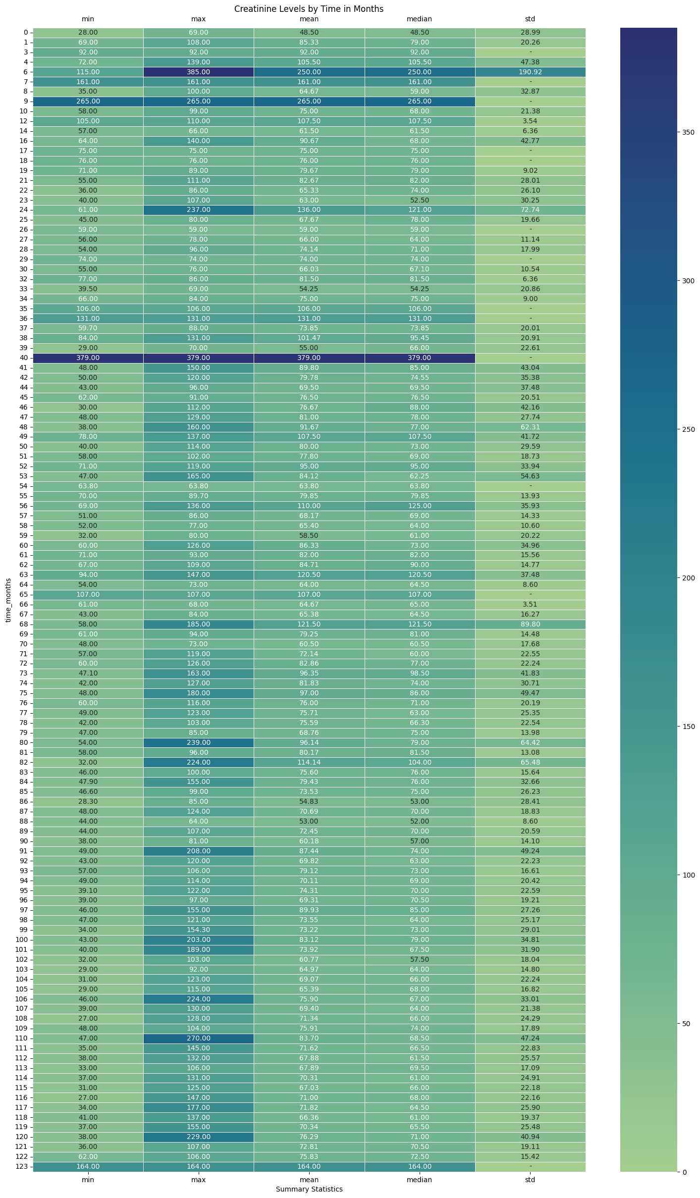
3.1 Serum Creatinine Levels (in $\mu mol/L$)
The dataset that the authors have furnished measures SCr in $\mu mol/L$ as opposed to $mg/dL$.
plt.figure(figsize=(18, 30))
sns.heatmap(
    df_eda.groupby("time_months")["creatinine"]
    .agg(["min", "max", "mean", "median", "std"])
    .fillna(0),
    annot=True,
    linewidths=0.5,
    fmt=".2f",
    cmap="crest",
)

# Replace 0s with "-" in the annotations.
for text in plt.gca().texts:
    if text.get_text() == "0.00":
        text.set_text("-")

# Set the title and move the x-axis to the top
plt.title("Creatinine Levels by Time in Months")

# Additional option: Rotate the x-axis labels if needed
plt.xticks(rotation=0)
plt.xlabel("Summary Statistics")
plt.tick_params(labeltop=True, labelbottom=True)
plt.savefig(os.path.join(image_path, "creatinine_levels_crosstab.svg"))
plt.show()
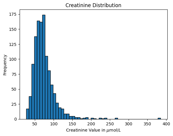
df_eda["creatinine"].hist(bins=50, edgecolor="black", grid=False)
plt.title("Creatinine Distribution")
plt.xlabel("Creatinine Value in $\mu mol/L$")
plt.ylabel("Frequency")
plt.savefig(os.path.join(image_path, "creatinine_hist.svg"))
plt.show()
df_eda["creatinine"].describe().to_frame().T
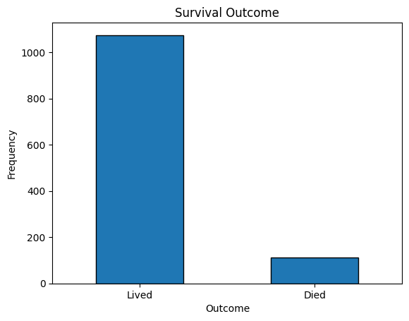
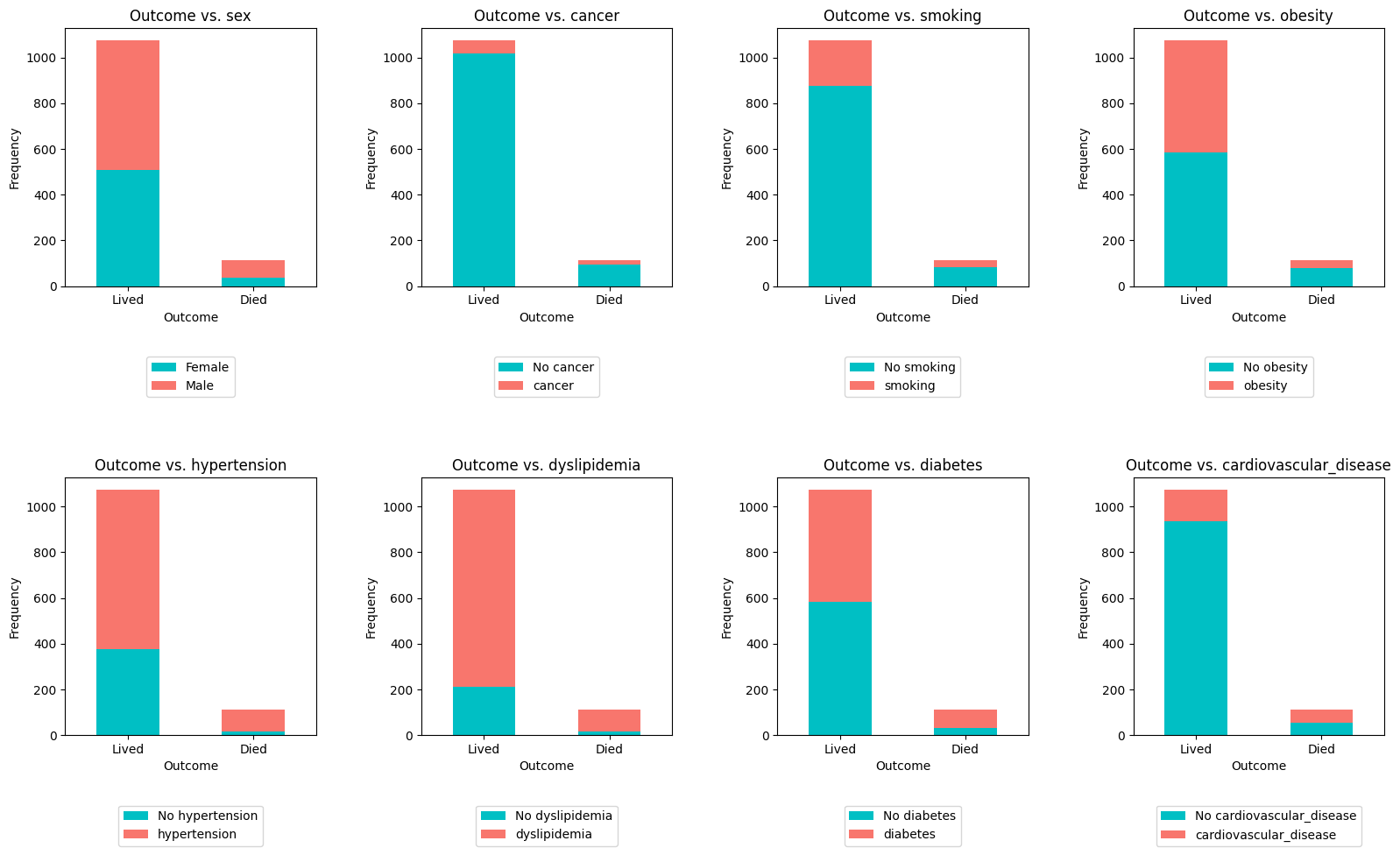
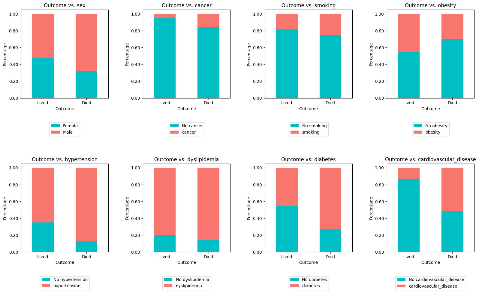
3.2 Survivability by Feature
ax = df_eda["outcome"].value_counts().plot(kind="bar", rot=0, edgecolor="black")
new_labels = ["Lived", "Died"]
ax.set_xticklabels(new_labels)
plt.title("Survival Outcome")
plt.xlabel("Outcome")
plt.ylabel("Frequency")
plt.savefig(os.path.join(image_path, "survival_outcome.svg"))
plt.show()
print()
print(
    df_eda["outcome"].value_counts().rename({0: "Lived", 1: "Died"}),
)
bar_list = df_eda.columns.to_list()
bar_list_remove = ["time_months", "outcome", "creatinine"]
bar_list = [item for item in bar_list if item not in bar_list_remove]
bar_list
crosstab_plot(
    df=df_eda,
    sub1=2,
    sub2=4,
    x=16,
    y=10,
    list_name=bar_list,
    label1="Lived",
    label2="Died",
    col1="sex",
    item1="Female",
    item2="Male",
    bbox_to_anchor=(0.5, -0.25),
    w_pad=4,
    h_pad=4,
    crosstab_option=True,
    image_path=image_path,
    string="outcome_by_feature.svg",
)
crosstab_plot(
    df=df_eda,
    sub1=2,
    sub2=4,
    x=16,
    y=10,
    list_name=bar_list,
    label1="Lived",
    label2="Died",
    col1="sex",
    item1="Female",
    item2="Male",
    bbox_to_anchor=(0.5, -0.25),
    w_pad=4,
    h_pad=4,
    crosstab_option=False,
    image_path=image_path,
    string="outcome_by_feature_normalized.svg",
)
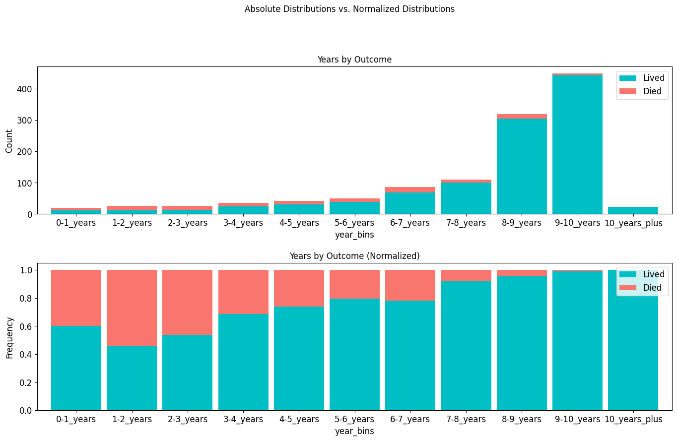
outcome_by_years = pd.crosstab(
    df_eda["year_bins"], df_eda["outcome"], margins=True, margins_name="Total_Count"
).rename(
    columns={0: "Lived", 1: "Died"},
)
outcome_by_years["Lived_%"] = round(
    outcome_by_years["Lived"] / outcome_by_years["Total_Count"] * 100, 2
)
outcome_by_years["Died_%"] = round(
    outcome_by_years["Died"] / outcome_by_years["Total_Count"] * 100, 2
)
outcome_by_years["Total_%"] = outcome_by_years["Lived_%"] + outcome_by_years["Died_%"]
outcome_by_years
stacked_plot(
    x=16,
    y=10,
    p=10,
    df=df_eda,
    col="year_bins",
    truth="outcome",
    condition=1,
    kind="bar",
    ascending=False,
    width=0.9,
    rot=0,
    string="Years",
    custom_order=[
        "0-1_years",
        "1-2_years",
        "2-3_years",
        "3-4_years",
        "4-5_years",
        "5-6_years",
        "6-7_years",
        "7-8_years",
        "8-9_years",
        "9-10_years",
        "10_years_plus",
    ],
    legend_labels=["Lived", "Died"],
    image_path=image_path,
    img_string="years_by_outcome.svg",
)
4 Modeling: Kidney_UAE
# paths to files
data_original = "/content/drive/MyDrive/kidney_uae/data/df_original/"
data_years = "/content/drive/MyDrive/kidney_uae/data/df_years/"
# save out the split datasets to separate parquet files
X_train = pd.read_parquet(os.path.join(data_original, "X_train.parquet"))
X_test = pd.read_parquet(os.path.join(data_original, "X_test.parquet"))
y_train = pd.read_parquet(os.path.join(data_original, "y_train.parquet"))
y_test = pd.read_parquet(os.path.join(data_original, "y_test.parquet"))
df_train = pd.read_parquet(os.path.join(data_original, "df_train.parquet"))
df_test = pd.read_parquet(os.path.join(data_original, "df_test.parquet"))
df = pd.read_parquet(os.path.join(data_original, "df_original.parquet"))
df_eda = pd.read_parquet(os.path.join(eda_path, "df_eda.parquet"))
## CPH-related joins to parse in "time_years" column and drop "time_months" col.
cph_train = df_train.join(df_eda["time_years"], on="id", how="inner").drop(
    columns=["time_months"]
)
cph_test = df_test.join(df_eda["time_years"], on="id", how="inner").drop(
    columns=["time_months"]
)
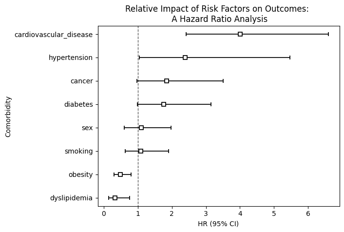
4.1 Cox Proportional Hazards (CPH) Model
# Instantiate the CoxPHFitter
cph = CoxPHFitter(
    baseline_estimation_method="breslow",
)

# Fit the model with additional options for the optimization routine
cph.fit(
    cph_train,
    duration_col="time_years",
    event_col="outcome",
    weights_col="creatinine",
    robust=True,
    show_progress=True,
)
# To evaluate the model, we will use the predict method on the test set and then
# calculate the concordance index
cph_train_score = cph.score(cph_train, scoring_method="concordance_index")
cph_validation_score = cph.score(cph_train, scoring_method="concordance_index")

cph_train_score, cph_validation_score
# print the summary of the model
# Print the summary of the model
cph.print_summary()
# Plot the results of the cph model with hazards ratios
cph.plot(hazard_ratios=True)
plt.title("Relative Impact of Risk Factors on Outcomes: \n A Hazard Ratio Analysis")
plt.ylabel("Comorbidity")
plt.savefig(
    os.path.join(image_path, "cph_hazard_ratios.svg"),
    bbox_inches="tight",
    dpi=300,
)
plt.show()
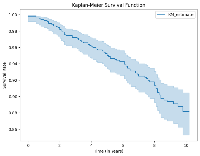
4.1.1 Kaplan-Meier Estimates
# Instantiate the Kaplan-Meier fitter
kmf = KaplanMeierFitter()

# Fit the data
kmf.fit(durations=cph_train["time_years"], event_observed=cph_train["outcome"])

# Plot the Kaplan-Meier estimate of the survival function
kmf.plot_survival_function(figsize=(8, 6))

plt.title("Kaplan-Meier Survival Function")
plt.xlabel("Time (in Years)")
plt.ylabel("Survival Rate")
plt.savefig(os.path.join(image_path, "kaplan_meier.svg"))
plt.show()  # Show the plot
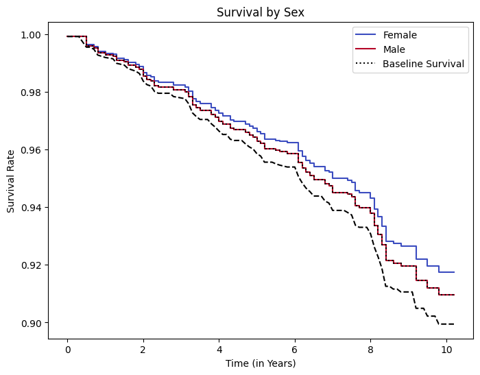
4.1.2 Partial Effects on Outcome
covariate = "sex"
# Then you define the values of the covariate you're interested in examining.
# For instance, if 'age' ranges from 20 to 70, you might choose a few key values within this range
values_of_interest = [0, 1]
labels = ["Female", "Male"]

# Generate the plot
ax = cph.plot_partial_effects_on_outcome(
    covariates=covariate, values=values_of_interest, cmap="coolwarm"
)

# Change the figure size here by accessing the figure object that 'ax' belongs to
ax.figure.set_size_inches(8, 6)

# Plot the baseline survival
cph.baseline_survival_.plot(
    ax=ax, color="black", linestyle="--", label="Baseline Survival"
)

# Manually construct the labels list including the baseline survival
labels_with_baseline = labels + ["Baseline Survival"]

# Retrieve the lines that have been plotted (which correspond to 'values_of_interest')
lines = ax.get_lines()

ax.set_title("Survival by Sex")
ax.set_xlabel("Time (in Years)")
ax.set_ylabel("Survival Rate")
ax.legend(lines, labels_with_baseline)  # Update the legend to include all lines
plt.savefig(os.path.join(image_path, "partial_effects_on_outcomes.svg"))
plt.show()  # Show the plot
4.2 Customized Machine Learning Algorithms
rstate = 222 # random state for reproducibility
# untuned models
# lr = LogisticRegression(class_weight="balanced", random_state=rstate)
# svm = SVC(class_weight="balanced", probability=True, random_state=rstate)
# rf = RandomForestClassifier(class_weight="balanced", random_state=rstate)
# et = ExtraTreesClassifier(class_weight="balanced", random_state=rstate)
# Define pipelines and parameter grids for each model
# Pipelines define a sequence of data processing steps followed by a model
# Each pipeline begins with feature scaling using StandardScaler to standardize
# the data

# Logistic regression with balanced class weight
# Standardize features by removing the mean and scaling to unit variance
pipeline_lr = Pipeline(
    [
        ("scaler", StandardScaler()),  # Standardize features
        ("lr", LogisticRegression(class_weight="balanced", random_state=rstate)),
    ]
)

# SVM with balanced class weight
pipeline_svm = Pipeline(
    [
        ("scaler", StandardScaler()),  # Standardize features
        ("svm", SVC(class_weight="balanced", probability=True, random_state=rstate)),
    ]
)

# Random forest with balanced class weight
pipeline_rf = Pipeline(
    [
        ("rf", RandomForestClassifier(class_weight="balanced", random_state=rstate)),
    ]
)

# Define the Extra Trees pipeline; Extra Trees with balanced class weight
pipeline_et = Pipeline(
    [
        ("et", ExtraTreesClassifier(class_weight="balanced", random_state=rstate)),
    ]
)

# Define the parameter grids for each model. The keys are prefixed with the
# model's name from the pipeline followed by a double underscore to specify
# parameter names for hyperparameter tuning.

# Parameter grid for the Logistic Regression model
param_grid_lr = {
    "lr__C": [0.001, 0.01, 0.1, 1, 10],  # Inverse of regularization strength
    "lr__solver": ["liblinear", "saga"],  # Algorithm in the optimization problem
    "lr__n_jobs": [-1],  # Number of CPU cores used when parallelizing over classes
}

# Parameter grid for the SVM model
param_grid_svm = {
    "svm__C": [0.1, 1, 10],  # Penalty parameter C of the error term
    "svm__kernel": ["linear", "poly", "rbf", "sigmoid"],  # kernel type
}

# Parameter grid for the Random Forest model
param_grid_rf = {
    "rf__n_estimators": [50, 100, 200, 500],  # The number of trees in the forest
    "rf__max_depth": [None, 10, 20, 30],  # The maximum depth of the tree
    "rf__min_samples_split": [2, 5, 10],  # min no. of samp. to split internal node
    "rf__n_jobs": [-1],  # The number of jobs to run in parallel
}

# Parameter grid for the Extra Trees model
param_grid_et = {
    "et__n_estimators": [200, 500, 1000],  # The number of trees in the forest
    "et__max_depth": [None, 10, 20, 30],  # The maximum depth of the tree
    "et__min_samples_split": [2, 5, 10],  # min no. of samp. to split internal node
    "et__n_jobs": [-1],  # The number of jobs to run in parallel
}

# GridSearchCV is set up for each model, defining cross-validation (cv) strategy,
# scoring metric, and verbosity
grid_search_lr = GridSearchCV(
    pipeline_lr,
    param_grid_lr,
    cv=5,
    scoring="accuracy",
    verbose=1,
)
grid_search_svm = GridSearchCV(
    pipeline_svm,
    param_grid_svm,
    cv=5,
    scoring="accuracy",
    verbose=1,
)
grid_search_rf = GridSearchCV(
    pipeline_rf,
    param_grid_rf,
    cv=5,
    scoring="accuracy",
    verbose=1,
)
grid_search_et = GridSearchCV(
    pipeline_et,
    param_grid_et,
    cv=5,
    scoring="accuracy",
    verbose=1,
)
4.2.1 Fitting Models Without Calibration
model_list = [
    ("grid_search_lr", grid_search_lr),
    ("grid_search_svm", grid_search_svm),
    ("grid_search_rf", grid_search_rf),
    ("grid_search_et", grid_search_et),
]

non_calibrated_probas_dict = {}

for name, model in tqdm(model_list, desc="Fitting models"):
    print(f"\nFitting {name}...")
    model.fit(
        X_train, y_train
    )  # This fits GridSearchCV which in turn finds the best estimator
    print(f"\nBest parameters for {name}: \n{model.best_params_}")

    # Predictions and probabilities from the calibrated model
    model_scores = model.predict(X_test)
    model_probas = model.predict_proba(X_test)[:, 1]

    # Storing scores and probabilities in probas_dict
    non_calibrated_probas_dict[name + "_score"] = model_scores
    non_calibrated_probas_dict[name + "_proba"] = model_probas
4.2.2 Fitting Models With Calibration
calibrated_models = {}
probas_dict = {}

for name, model in tqdm(model_list, desc="Fitting models"):
    print(f"\nFitting {name}...")
    model.fit(
        X_train, y_train
    )  # This fits GridSearchCV which in turn finds the best estimator
    print(f"\nBest parameters for {name}: \n{model.best_params_}")

    # Create a calibrated classifier from the best estimator of the grid search
    calibrated_clf = CalibratedClassifierCV(
        model.best_estimator_,
        method="isotonic",
        cv=5,
    ).fit(X_train, y_train)

    # Store the calibrated model for potential later use
    calibrated_models[name] = calibrated_clf

    # Predictions and probabilities from the calibrated model
    model_scores = calibrated_clf.predict(X_test)
    model_probas = calibrated_clf.predict_proba(X_test)[:, 1]

    # Storing scores and probabilities in probas_dict
    probas_dict[name + "_score"] = model_scores
    probas_dict[name + "_proba"] = model_probas
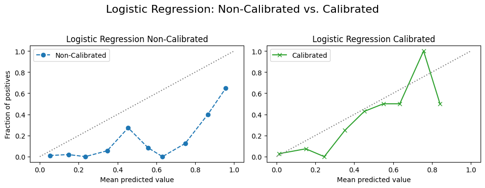
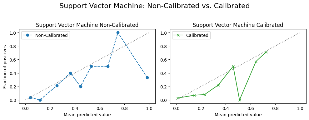
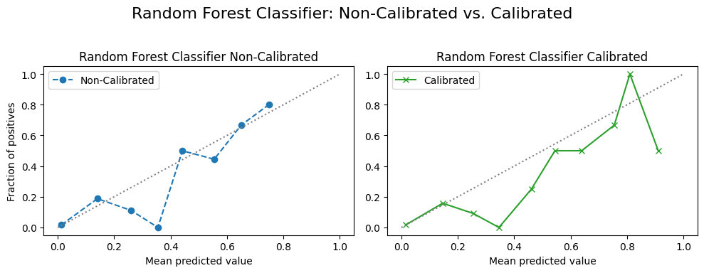
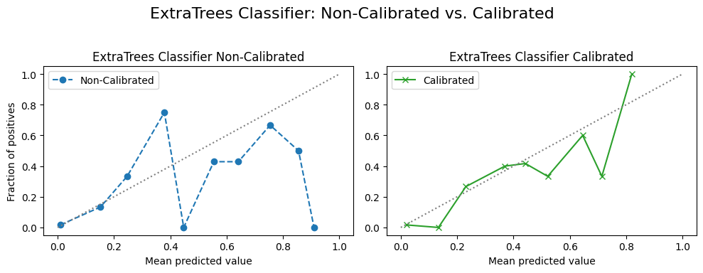
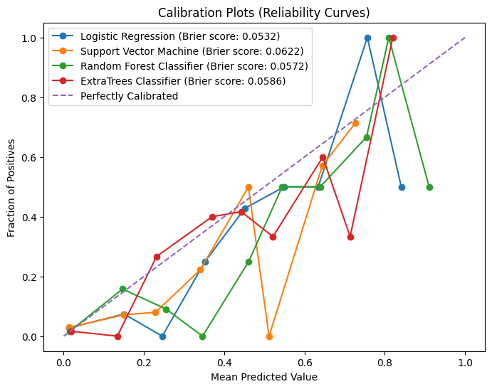
4.2.3 Calibration Curves
custom_titles = {
    "grid_search_lr": "Logistic Regression",
    "grid_search_svm": "Support Vector Machine",
    "grid_search_rf": "Random Forest Classifier",
    "grid_search_et": "ExtraTrees Classifier",
}

# Loop through each model to create a side-by-side plot for non-calibrated and
# calibrated models
for name, model in model_list:
    fig, (ax1, ax2) = plt.subplots(
        1, 2, figsize=(10, 4)
    )  # figsize adjusted for two subplots side by side

    # Non-Calibrated Model
    prob_true_non_calib, prob_pred_non_calib = calibration_curve(
        y_test,
        non_calibrated_probas_dict[f"{name}_proba"],
        n_bins=10,
        strategy="uniform",
    )
    ax1.plot(
        prob_pred_non_calib,
        prob_true_non_calib,
        marker="o",
        linestyle="--",
        color="tab:blue",
        label="Non-Calibrated",
    )
    ax1.plot([0, 1], [0, 1], linestyle=":", color="gray")
    ax1.set_title(f"{custom_titles[name]} Non-Calibrated")  # Use custom title
    ax1.set_xlabel("Mean predicted value")
    ax1.set_ylabel("Fraction of positives")
    ax1.legend()

    # Calibrated Model
    prob_true_calib, prob_pred_calib = calibration_curve(
        y_test, probas_dict[f"{name}_proba"], n_bins=10, strategy="uniform"
    )
    ax2.plot(
        prob_pred_calib,
        prob_true_calib,
        marker="x",
        linestyle="-",
        color="tab:green",
        label="Calibrated",
    )
    ax2.plot([0, 1], [0, 1], linestyle=":", color="gray")
    ax2.set_title(f"{custom_titles[name]} Calibrated")  # Use custom title
    ax2.set_xlabel("Mean predicted value")
    ax2.legend()

    fig.suptitle(
        f"{custom_titles[name]}: Non-Calibrated vs. Calibrated",
        fontsize=16,
    )
    plt.tight_layout(rect=[0, 0.03, 1, 0.95])
    filename = f"{name}_non_calibrated_vs_calibrated.svg"
    filepath = os.path.join(image_path, filename)

    plt.savefig(filepath)  # Save the figure with the unique filename
    plt.show()
model_dict = {
    "Logistic Regression": probas_dict["grid_search_lr_proba"],
    "Support Vector Machine": probas_dict["grid_search_svm_proba"],
    "Random Forest Classifier": probas_dict["grid_search_rf_proba"],
    "ExtraTrees Classifier": probas_dict["grid_search_et_proba"],
}

plot_calibration_curves(
    y_true=y_test,
    model_dict=model_dict,
    image_path=image_path,
    img_string="calibration_curves.svg",
)
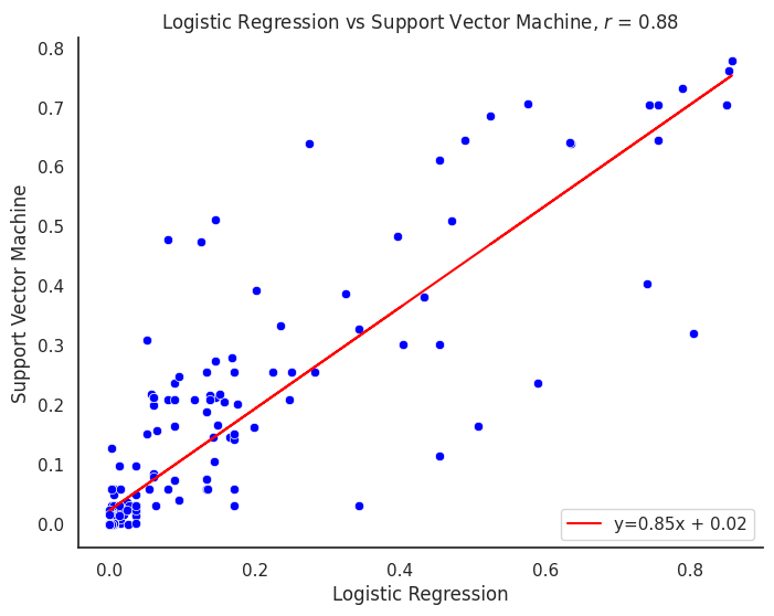
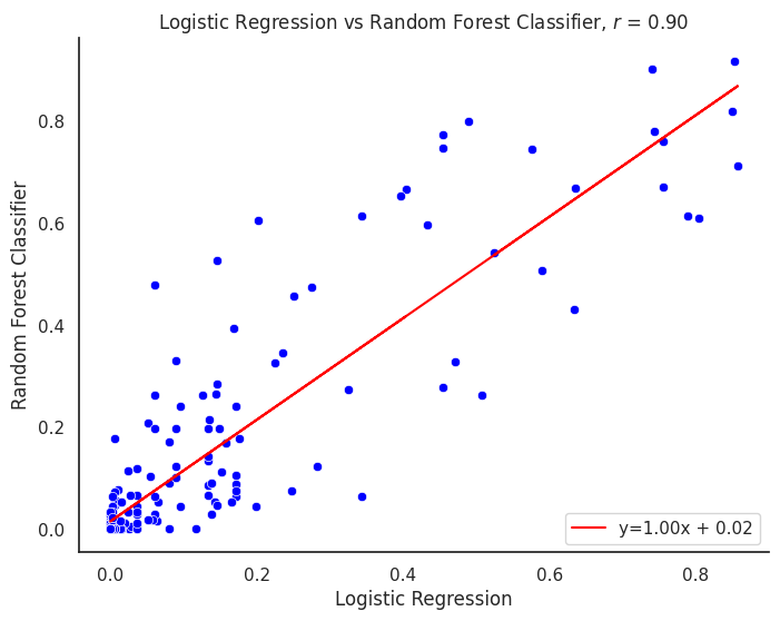
4.3 Performance Assessment
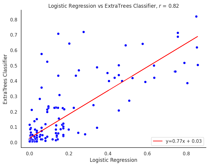
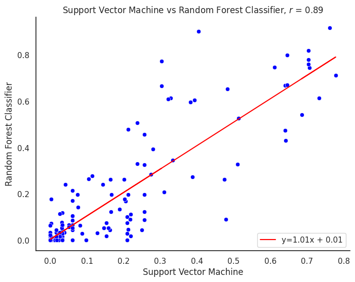
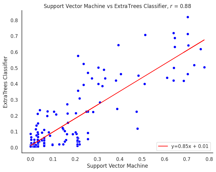
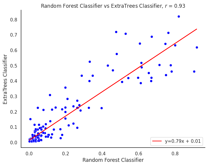
4.3.1 Model Prediction Comparisons
proba_df = pd.DataFrame(
    {key: value for key, value in probas_dict.items() if key.endswith("proba")}
)
x_cols = [col for col in proba_df if not "grid_search_rf_proba" in col]
y_col = "grid_search_rf_proba"
# Now plot scatter plots for each pair of columns
pairwise_combinations = list(combinations(proba_df.columns, 2))

# Set up the matplotlib figure
sns.set(style="white")

# Since we need to plot each scatterplot separately, let's iterate over the
# combinations again and plot them one by one.
# Iterate over each pair of columns
for col1, col2 in pairwise_combinations:
    plt.figure(figsize=(8, 6))

    # Find custom title for ea. column, if not found, use the column name itself
    title1 = custom_titles.get(col1.replace("_proba", ""), col1)
    title2 = custom_titles.get(col2.replace("_proba", ""), col2)

    # Set the plot title, x-label, and y-label using the custom titles
    plot_title = f"{title1} vs {title2}"
    x_label = title1
    y_label = title2

    corr_model = proba_df[col1].corr(proba_df[col2])
    m, b = np.polyfit(proba_df[col1], proba_df[col2], 1)
    line_label = f"y={m:.02f}x + {b:.02f}"
    plt.plot(proba_df[col1], m * proba_df[col1] + b, color="red", label=line_label)

    sns.scatterplot(data=proba_df, x=col1, y=col2, color="#0000ff")
    plt.title(f"{plot_title}, $r$ = {corr_model:.2f}")
    plt.xlabel(x_label)
    plt.ylabel(y_label)
    plt.legend(loc="lower right")
    sns.despine()  # Optionally remove the top and right spines
    plt.savefig(os.path.join(image_path, f"{plot_title}.svg"))
    plt.show()
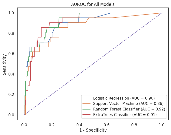
4.3.2 AUROC Curves by Model
plt.figure(figsize=(8, 6))
for name, proba in model_dict.items():
    fpr, tpr, _ = roc_curve(y_test, proba)  # calculate values for TPR, FPR
    auc_models = auc(fpr, tpr)  # calculate the auc for all models
    plt.plot(fpr, tpr, label=f"{name} (AUC = {auc_models:.2f})")  # plot the ROC AUC

plt.plot([0, 1], [0, 1], "--")
plt.title("AUROC for All Models")
plt.xlabel("1 - Specificity")
plt.ylabel("Sensitivity")
plt.legend()
plt.savefig(os.path.join(image_path, "roc_auc_models.svg"))
plt.show()
metrics_df = evaluate_model_metrics(
    y_test=y_test,
    model_dict=model_dict,
    threshold=0.5,
)
metrics_df
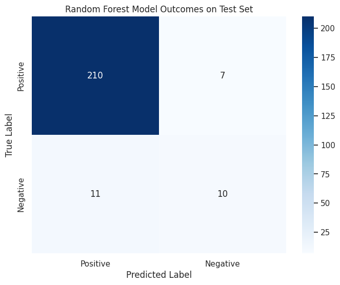
4.3.3 Confusion Matrix (Random Forest Model)
# Extract the feature names from X_train
feature_names = X_train.columns.to_list()

# Extract the best estimator from your grid_search_rf
# This indexes into grid_search_rf; adjust if necessary
best_rf_model = model_list[2][1].best_estimator_
rf_model = best_rf_model.named_steps["rf"]
y_pred = best_rf_model.predict(X_test)

# Calculate the confusion matrix
conf_matrix = confusion_matrix(y_test, y_pred)

# Plot the confusion matrix
plt.figure(figsize=(8, 6))
sns.heatmap(
    conf_matrix,
    annot=True,
    fmt="d",
    cmap="Blues",
    xticklabels=["Positive", "Negative"],
    yticklabels=["Positive", "Negative"],
)
plt.title("Random Forest Model Outcomes on Test Set")
plt.xlabel("Predicted Label")
plt.ylabel("True Label")
plt.savefig(os.path.join(image_path, "rf_confusion_matrix.svg"))
plt.show()
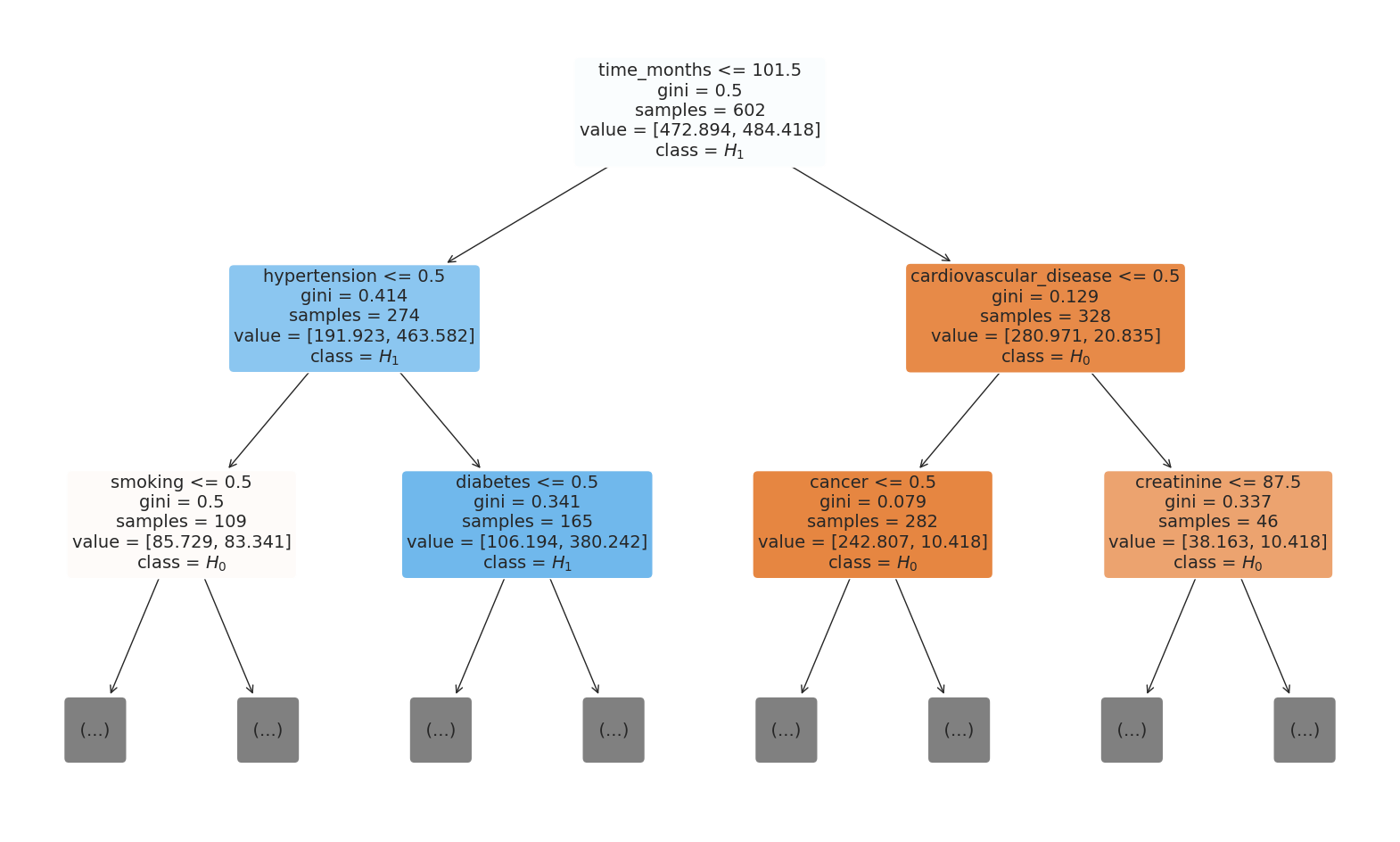
4.3.4 Decision Tree from Random Forest Model
# Choose the tree you want to plot (e.g., the first tree)
chosen_tree = rf_model.estimators_[0]

# Plot the tree with a limited depth
plt.figure(figsize=(20, 12))

# Specify the class names as a list
class_names = ["$H_0$", "$H_1$"]

plot_tree(
    chosen_tree,
    filled=True,
    rounded=True,
    class_names=class_names,
    max_depth=2,  # Set the maximum depth to something low
    feature_names=X_test.columns,
    fontsize=14,
)
plt.savefig(
    os.path.join(image_path, "random_forest_viz.svg"), bbox_inches="tight", dpi=300
)
plt.show()
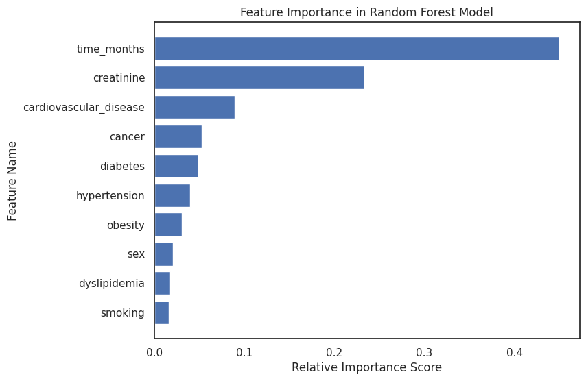
4.3.5 Random Forest Feature Importances
# Access the feature importances
importances = rf_model.feature_importances_
indices = np.argsort(importances)[::-1]
sorted_names = [feature_names[i] for i in indices]

# Plot
plt.figure(figsize=(8, 6))
plt.title("Feature Importance in Random Forest Model")
plt.barh(range(len(importances)), importances[indices])
plt.yticks(range(len(importances)), sorted_names)
plt.gca().invert_yaxis()  # To display the highest importance at the top
plt.xlabel("Relative Importance Score")
plt.ylabel("Feature Name")
plt.savefig(
    os.path.join(image_path, "rf_feat_importance.svg"), bbox_inches="tight", dpi=300
)
plt.show()
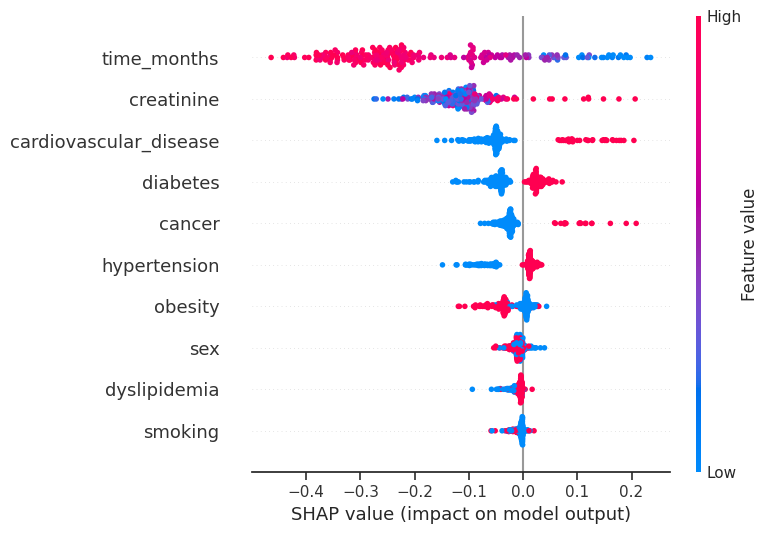
4.3.6 SHAP Values
# Initialize the SHAP Explainer with your Random Forest model
explainer = shap.TreeExplainer(rf_model)

# Compute SHAP values for your test set
shap_values = explainer.shap_values(X_test)

# Selecting SHAP values for the positive class
shap_values_positive_class = shap_values[:, :, 1]

# Now, shap_values_positive_class should have the correct shape
shap.summary_plot(
    shap_values_positive_class, X_test, feature_names=feature_names, show=False,
)

plt.savefig(
    os.path.join(image_path, "shap_value_importance.svg"), bbox_inches="tight",
    dpi=300,
)

plt.show()
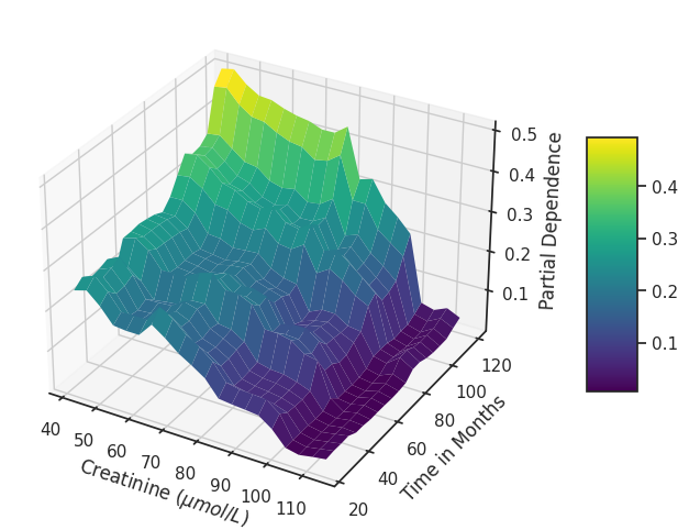
4.3.7 Partial Dependence
plot_3d_partial_dependence(
    model=rf_model,
    dataframe=X_test,  # or any DataFrame you choose
    feature_names_list=["creatinine", "time_months"],
    x_label="Creatinine ($\mu mol/L$)",
    y_label="Time in Months",
    z_label="Partial Dependence",
    title="",
    horizontal=0.99,
    depth=-1.25,
    vertical=0.99,
    html_file_path=image_path,
    html_file_name="interactive_partial_dependence.html",
    interactive=False,
    static=True,  # Set this to True to generate the static plot as well
    matplotlib_colormap="viridis",
    plotly_colormap="Viridis",
    zoom_out_factor=1.7,
)

# After the function call, save the current figure
plt.savefig(os.path.join(image_path, "static_partial_dependence.svg"),
            bbox_inches="tight",)

# If you want to display the plot as well
plt.show()
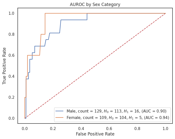
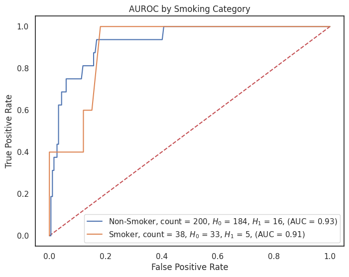
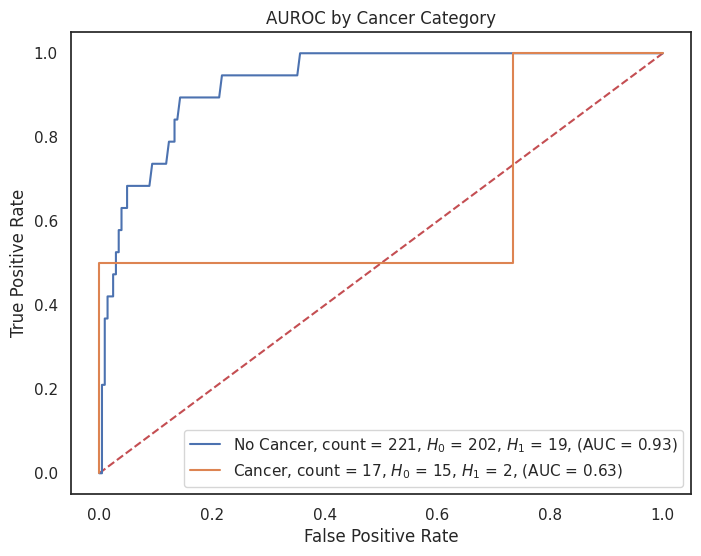
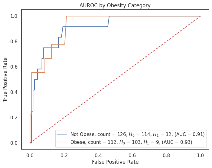
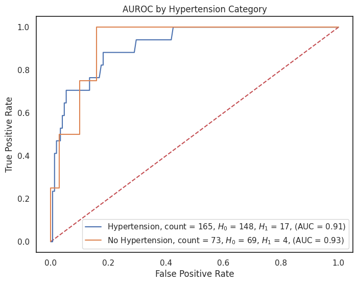
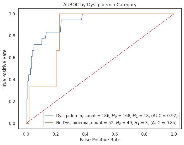
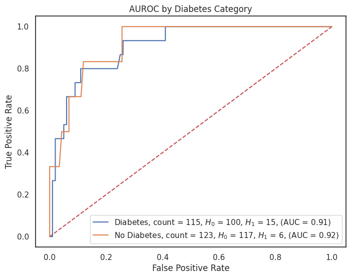
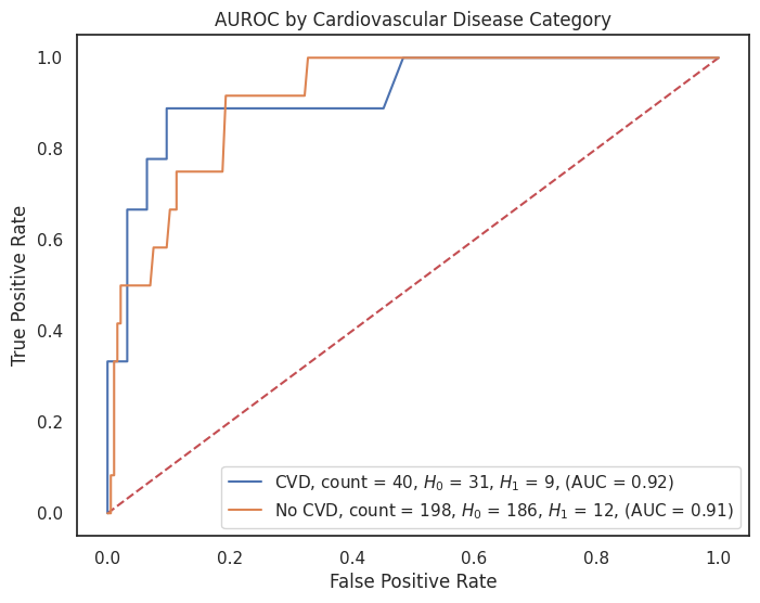
4.3.8 AUROC by Feature
# Dictionary of model predictions
model_predictions = probas_dict["grid_search_rf_proba"]

# Dictionary of custom category labels for each column
category_label_dict = {
    "sex": {1: "Male", 0: "Female"},
    "smoking": {1: "Smoker", 0: "Non-Smoker"},
    "cancer": {1: "Cancer", 0: "No Cancer"},
    "obesity": {1: "Obese", 0: "Not Obese"},
    "hypertension": {1: "Hypertension", 0: "No Hypertension"},
    "dyslipidemia": {1: "Dyslipidemia", 0: "No Dyslipidemia"},
    "diabetes": {1: "Diabetes", 0: "No Diabetes"},
    "cardiovascular_disease": {1: "CVD", 0: "No CVD"}
    # Add more feature_label pairs as needed
}

# Loop over each feature you want to create a ROC plot for

for feature, category_labels in category_label_dict.items():
    title = f"AUROC by {feature.replace('_', ' ').title()} Category"
    plt.figure(figsize=(8, 6))
    plot_roc_curves_by_category(
        X_test=X_test,
        y_test=y_test,
        predictions=model_predictions,
        feature=feature,
        category_labels=category_labels,
        outcome="outcome",
        title=title,
        image_path=image_path,
        img_string=f"auc_roc_by_{feature}.svg",
    )
4.4 Save Best Model's Predictions
model_df = pd.DataFrame(index=X_test.index)

# Add the scores to the DataFrame
for name, values in probas_dict.items():
    if name.endswith("_score"):
        model_df[name] = values
    elif name.endswith("_proba"):
        model_df[name] = values
pd.DataFrame(model_df["grid_search_rf_score"]).to_parquet(
    os.path.join(data_original, "rf_score.parquet")
)
4.5 Bias & Fairness Analysis
# read the necessary parquet files from paths
df = pd.read_parquet(os.path.join(data_original, "df_original.parquet"))
y_test = pd.read_parquet(os.path.join(data_original, "y_test.parquet"))
rf_score = pd.read_parquet(os.path.join(data_original, "rf_score.parquet"))
df_audit = df.copy(deep=True)
df_audit["sex_cat"] = df_audit["sex"].apply(lambda x: "Male" if x == 1 else "Female")
audit_sex = y_test.join(rf_score, on="id", how="inner").join(
    df_audit["sex_cat"], on="id", how="inner"
)
audit_sex.head()
audit_sex.shape
audit_sex = move_column_before(
    df=audit_sex, target_column="grid_search_rf_score", before_column="sex_cat",
)
audit_sex.shape
audit = Audit(df=audit_sex, score_column="grid_search_rf_score",
              label_column="outcome",)
audit.audit()
audit.confusion_matrix
audit.metrics.round(2)
audit.disparity_df.style
audit.disparities.style
metrics = ["fpr", "fdr", "pprev"]
disparity_tolerance = 1.25
audit_sex_groups = Audit(
    df=audit_sex,
    score_column="grid_search_rf_score",
    label_column="outcome",
    reference_groups={"sex_cat": "Male"},
)
audit_sex_groups.audit()
summary_plot_kidney = audit_sex_groups.summary_plot(
    metrics=metrics,
    fairness_threshold=disparity_tolerance,
)
summary_plot_kidney
disparity_plot_kidney = audit.disparity_plot(
    metrics=metrics, attribute="sex_cat", fairness_threshold=disparity_tolerance
)
disparity_plot_kidney
4.6 References
Al-Shamsi, S., Govender, R. D., & King, J. (2021). Predictive value of creatinine-based equations of kidney function in the long-term prognosis of United Arab Emirates patients with vascular risk. Oman medical journal, 36(1), e217. https://doi.org/10.5001/omj.2021.07
Al-Shamsi, S., Govender, R. D., & King, J. (2019). Predictive value of creatinine-based equations of kidney function in the long-term prognosis of United Arab Emirates patients with vascular risk [Dataset]. Mendeley Data, V1. https://data.mendeley.com/datasets/ppfwfpprbc/1