Appendix: Exploratory Data Analysis (EDA) and Preprocessing
Team 2 - Shpaner, Leonid; Oakes, Isabella, Lucban, Emanuel
Loading the requisite libraries
import pandas as pd
import numpy as np
import json

import matplotlib.pyplot as plt
import seaborn as sns
import plotly as ply
import random

from sklearn.preprocessing import OneHotEncoder, OrdinalEncoder, LabelEncoder, \
StandardScaler, Normalizer
from sklearn.model_selection import train_test_split
from sklearn.linear_model import BayesianRidge, LogisticRegression

# Enable Experimental
from sklearn.experimental import enable_iterative_imputer
from sklearn.impute import SimpleImputer, IterativeImputer
from sklearn import tree

import statsmodels.api as sm
from scipy import stats
from sklearn.metrics import confusion_matrix, plot_confusion_matrix,\
classification_report,accuracy_score

from sklearn import linear_model
from sklearn.svm import SVC

import warnings
warnings.filterwarnings('ignore')
Reading in and Inspecting the dataframe
coupons_df = pd.read_csv('https://archive.ics.uci.edu/ml/\
machine-learning-databases/00603/in-vehicle-coupon-recommendation.csv')
coupons_df.head()
coupons_df.dtypes
null_vals = pd.DataFrame(coupons_df.isna().sum(), columns=['Null Count'])
null_vals['Null Percent'] = (null_vals['Null Count'] / coupons_df.shape[0]) * 100
null_vals
EDA - Discovery
Renaming Columns
# Renaming the passanger column to 'passenger'
coupons_df = coupons_df.rename(columns={'passanger':'passenger'})

# Renaming the 'Y' column as our Target
coupons_df = coupons_df.rename(columns={'Y':'Target'})

# Binarizing Target Variable
coupons_df['Target'] = coupons_df['Target'].map({1 : 'yes', 0 : 'no'})

# Creating a new column of dummy var. for Binary Target (Response)
coupons_df['Response'] = coupons_df['Target'].map({'yes':1, 'no':0})
Removing Highly Correlated Predictors
correlation_matrix = coupons_df.corr()
correlated_features = set()

for i in range(len(correlation_matrix .columns)):
    for j in range(i):
        if abs(correlation_matrix.iloc[i, j]) > 0.8:
            colname = correlation_matrix.columns[i]
            correlated_features.add(colname)
print(correlated_features)
Mapping Important Categorical Features to Numerical Ones
print(coupons_df['education'].unique())
coupons_df['educ. level'] = coupons_df['education'].map(\
                            {'Some High School':1,
                             'Some college - no degree':2,
                             'Bachelors degree':3, 'Associates degree':4,
                             'High School Graduate':5,
                             'Graduate degree (Masters or Doctorate)':6})
# create new variable 'avg_income' based on income
inc = coupons_df['income'].str.findall('(\d+)')
coupons_df['avg_income'] = pd.Series([])

for i in range(0,len(inc)):
    inc[i] = np.array(inc[i]).astype(np.float)
    coupons_df['avg_income'][i] = sum(inc[i]) / len(inc[i])

print(coupons_df['avg_income'])
# Creating new age range column
print(coupons_df['age'].value_counts())
coupons_df['Age Range'] = coupons_df['age'].map({'below21':'21 and below',
                                                 '21':'21-25','26':'26-30',
                                                 '31':'31-35','36':'36-40',
                                                 '41':'41-45','46':'46-50',
                                                 '50plus':'50+'})
# Creating new age group column based on ordinal values
print(coupons_df['age'].value_counts())
coupons_df['Age Group'] = coupons_df['age'].map({'below21':1,
                                                 '21':2,'26':3,
                                                 '31':4,'36':5,
                                                 '41':6,'46':6,
                                                 '50plus':7})
# Numericizing Age variable by adding new column: 'ages'
coupons_df['ages'] = coupons_df['age'].map({'below21':20,
                                            '21':21,'26':26,
                                            '31':31,'36':36,
                                            '41':41,'46':46,
                                            '50plus':65})
# Changing coupon expiration to uniform # of hours
coupons_df['expiration'] = coupons_df['expiration'].map({'1d':24, '2h':2})
# Convert time to 24h military time
def convert_time(x):
    if x[-2:] == "AM":
        return int(x[0:-2]) % 12
    else:
        return (int(x[0:-2]) % 12) + 12

coupons_df['time'] = coupons_df['time'].apply(convert_time)
Selected Features by Target Response
print("\033[1m"+'Target Outcome by Age (Maximum Values):'+"\033[1m")

def target_by_age():
    target_yes = coupons_df.loc[coupons_df.Target == 'yes'].groupby(
                               ['Age Range'])[['Target']].count()
    target_yes.rename(columns={'Target':'Yes'}, inplace=True)

    target_no = coupons_df.loc[coupons_df.Target == 'no'].groupby(
                               ['Age Range'])[['Target']].count()
    target_no.rename(columns={'Target':'No'}, inplace=True)

    target_age = pd.concat([target_yes, target_no], axis = 1)
    target_age['Yes'] = target_age['Yes'].fillna(0)
    target_age['No'] = target_age['No'].fillna(0)
    target_age
    max = target_age.max()
    print(max)
    target_age.loc['Total'] = target_age.sum(numeric_only=True, axis=0)
    target_age['% of Total'] = round((target_age['Yes'] / (target_age['Yes'] \
                                                + target_age['No']))* 100, 2)
    return target_age.style.format("{:,.0f}")

target_by_age()
print("\033[1m"+'Target Outcome by Income (Maximum Values):'+"\033[1m")

def target_by_income():
    target_yes = coupons_df.loc[coupons_df.Target == 'yes'].\
    groupby(['avg_income'])[['Target']].count()
    target_yes.rename(columns={'Target':'Yes'}, inplace=True)

    target_no = coupons_df.loc[coupons_df.Target == 'no'].\
    groupby(['avg_income'])[['Target']].count()
    target_no.rename(columns={'Target':'No'}, inplace=True)

    target_inc = pd.concat([target_yes, target_no], axis = 1)
    target_inc['Yes'] = target_inc['Yes'].fillna(0)
    target_inc['No'] = target_inc['No'].fillna(0)
    target_inc
    max = target_inc.max()
    print(max)
    target_inc.loc['Total'] = target_inc.sum(numeric_only=True, axis=0)
    target_inc['% of Total'] = round((target_inc['Yes'] / (target_inc['Yes'] \
                                    + target_inc['No']))* 100, 2)
    return target_inc.style.format("{:,.0f}")

target_by_income()
Selected Features' Value Counts
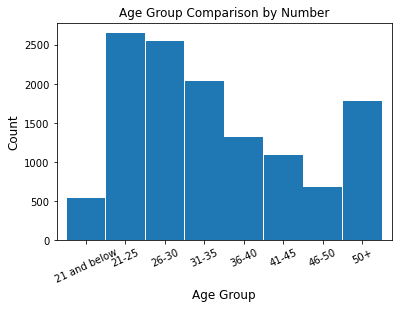
age_count = coupons_df['Age Range'].value_counts().reindex(["21 and below",
                                             "21-25", "26-30",
                                             "31-35","36-40",
                                             "41-45", "46-50",
                                             "50+"])
fig = plt.figure()
age_count.plot.bar(x ='lab', y='val', rot=0, width=0.98)
plt.title ('Age Group Comparison by Number', fontsize=12)
plt.xlabel('Age Group', fontsize=12)
plt.ylabel('Count', fontsize=12); plt.xticks(rotation = 25)
plt.show()
age_count
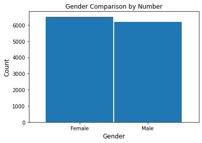
gender_count = coupons_df['gender'].value_counts()
fig = plt.figure()
gender_count.plot.bar(x ='lab', y='val', rot=0, width=0.99)
plt.title ('Gender Comparison by Number', fontsize=12)
plt.xlabel('Gender', fontsize=12)
plt.ylabel('Count', fontsize=12)
plt.show()
gender_count
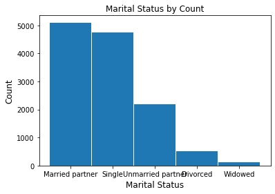
marital_coupons = coupons_df['maritalStatus'].value_counts()
fig = plt.figure()
marital_coupons.plot.bar(x ='lab', y='val', rot=0, width=0.98)
plt.title ('Marital Status by Count', fontsize=12)
plt.xlabel('Marital Status', fontsize=12)
plt.ylabel('Count', fontsize=12)
plt.show()
marital_coupons
print("\033[1m"+'Coupon Summary Statistics:'+"\033[1m")

def coupon_summary_stats():
    pd.options.display.float_format = '{:,.2f}'.format
    coupon_summary = pd.DataFrame(coupons_df).describe().transpose()
    cols_to_keep = ['mean', 'std', 'min', '25%', '50%','75%', 'max']
    coupon_summary = coupon_summary[cols_to_keep]
    stats_rename = coupon_summary.rename(columns={'count':'Count','min':'Minimum',
                                '25%':'Q1','50%':'Median','mean':'Mean','75%':
                                'Q3','std': 'Standard Deviation','max':'Maximum'})
    return stats_rename

coupon_summary_stats()
fig = plt.figure(figsize=(12, 8))
ax2 = fig.add_subplot(221); ax1 = fig.add_subplot(222)
fig.suptitle('Normalized vs. Absolute Distributions')

crosstabdest = pd.crosstab(coupons_df['destination'], coupons_df['Target'])
crosstabdestnorm = crosstabdest.div(crosstabdest.sum(1), axis=0)

plotdest = crosstabdest.plot(kind='bar',
                             stacked=True,
                             title='Destination and Target',
                             ax=ax1,
                             color=['#90CDBC', '#991857'])

plotdestnorm = crosstabdestnorm.plot(kind='bar',
                                     stacked=True,
                                     title='Destination and Target Normalized',
                                     ax=ax2,
                                     color=['#90CDBC', '#991857'])
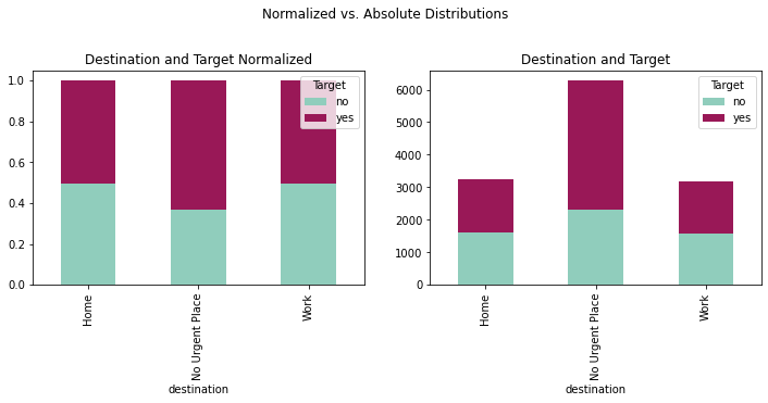
fig = plt.figure(figsize=(12,8))
ax2 = fig.add_subplot(221); ax1 = fig.add_subplot(222)
fig.suptitle('Normalized vs. Absolute Distributions')

crosstabpass = pd.crosstab(coupons_df['passenger'],coupons_df['Target'])
crosstabpassnorm = crosstabpass.div(crosstabpass.sum(1), axis = 0)
plotpass = crosstabpass.plot(kind='bar', stacked = True,
                             title = 'Passenger and Target',
                             ax = ax1, color = ['#90CDBC', '#991857'])
plotpassnorm = crosstabpassnorm.plot(kind='bar', stacked = True,
                                     title = 'Passenger and Target Normalized',
                                     ax = ax2, color = ['#90CDBC', '#991857'])
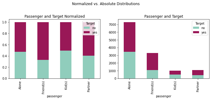
fig = plt.figure(figsize=(12,8))
ax2 = fig.add_subplot(221)
ax1 = fig.add_subplot(222)
fig.suptitle('Normalized vs. Absolute Distributions')

crosstabweat = pd.crosstab(coupons_df['weather'],coupons_df['Target'])
crosstabweatnorm = crosstabweat.div(crosstabweat.sum(1), axis=0)

plotweat = crosstabweat.plot(kind='bar', stacked = True,
                             title='Weather and Target',
                             ax=ax1, color=['#90CDBC', '#991857'])

plotweatnorm = crosstabweatnorm.plot(kind='bar', stacked = True,
                                     title='Weather and Target Normalized',
                                     ax=ax2, color=['#90CDBC', '#991857'])
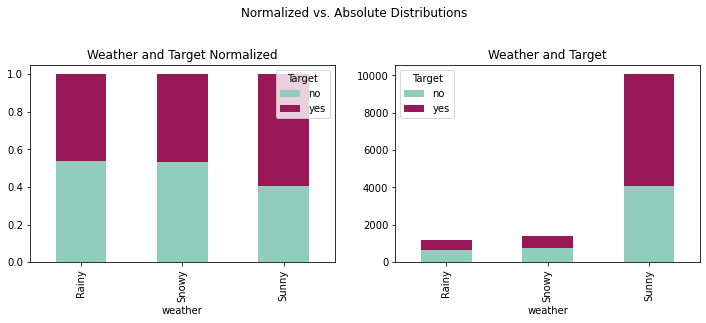
fig = plt.figure(figsize=(12,8))
ax2 = fig.add_subplot(221)
ax1 = fig.add_subplot(222)
fig.suptitle('Normalized vs. Absolute Distributions')

crosstabtemp = pd.crosstab(coupons_df['temperature'],coupons_df['Target'])
crosstabtempnorm = crosstabtemp.div(crosstabtemp.sum(1), axis = 0)

plottemp = crosstabtemp.plot(kind='bar', stacked = True,
                             title = 'Temperature and Target',
                             ax = ax1, color = ['#90CDBC', '#991857'])

plottempnorm = crosstabtempnorm.plot(kind='bar', stacked = True,
                                     title = 'Temperature and Target Normalized',
                                     ax = ax2, color = ['#90CDBC', '#991857'])
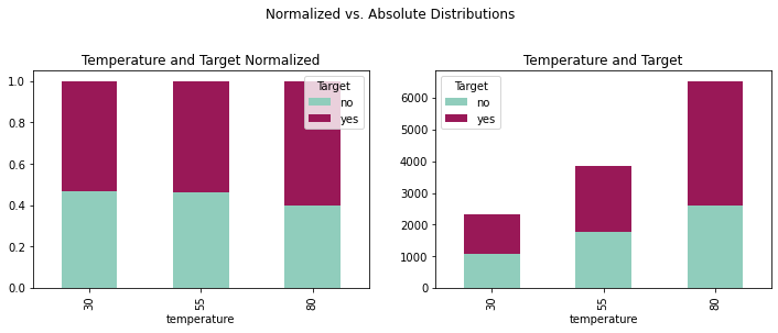
fig = plt.figure(figsize=(12,8))
ax2 = fig.add_subplot(221)
ax1 = fig.add_subplot(222)
fig.suptitle('Normalized vs. Absolute Distributions')

crosstabtime = pd.crosstab(coupons_df['time'],coupons_df['Target'])
crosstabtimenorm = crosstabtime.div(crosstabtime.sum(1), axis = 0)

plottime = crosstabtime.plot(kind='bar',
                             stacked=True,
                             title='Time and Target',
                             ax=ax1,
                             color=['#90CDBC', '#991857'])
plottimenorm = crosstabtimenorm.plot(kind='bar',
                                     stacked=True,
                                     title='Time and Target Normalized',
                                     ax=ax2,
                                     color=['#90CDBC', '#991857'])
fig = plt.figure(figsize=(12,8))
ax2 = fig.add_subplot(221)
ax1 = fig.add_subplot(222)
# fig.suptitle('Normalized vs. Absolute Distributions')

crosstabcoup = pd.crosstab(coupons_df['coupon'],coupons_df['Target'])
crosstabcoupnorm = crosstabcoup.div(crosstabcoup.sum(1), axis = 0)

plotcoup = crosstabcoup.plot(kind='bar', stacked = True,
                             title = 'Coupon and Target',
                             ax = ax1, color = ['#90CDBC', '#991857'])

plotcoupnorm = crosstabcoupnorm.plot(kind='bar', stacked = True,
                                     title = 'Coupon and Target Normalized',
                                     ax = ax2, color = ['#90CDBC', '#991857'])
fig = plt.figure(figsize=(12,8))
ax2 = fig.add_subplot(221); ax1 = fig.add_subplot(222)
fig.suptitle('Normalized vs. Absolute Distributions')

crosstabexpi = pd.crosstab(coupons_df['expiration'],coupons_df['Target'])
crosstabexpinorm = crosstabexpi.div(crosstabexpi.sum(1), axis = 0)
plotexpi = crosstabexpi.plot(kind='bar', stacked = True,
                             title = 'Expiration and Target', ax = ax1,
                             color = ['#90CDBC', '#991857'])
plotexpinorm = crosstabexpinorm.plot(kind='bar', stacked = True,
                                     title = 'Expiration and Target Normalized',
                                     ax = ax2, color = ['#90CDBC', '#991857'])
fig = plt.figure(figsize=(12,8))
ax2 = fig.add_subplot(221)
ax1 = fig.add_subplot(222)
fig.suptitle('Normalized vs. Absolute Distributions')

crosstabgender = pd.crosstab(coupons_df['gender'],coupons_df['Target'])
crosstabgendernorm = crosstabgender.div(crosstabgender.sum(1), axis = 0)

plotgender = crosstabgender.plot(kind='bar', stacked = True,
                                 title = 'Gender and Target',
                                 ax = ax1, color = ['#90CDBC', '#991857'])


plotgendernorm = crosstabgendernorm.plot(kind='bar', stacked = True,
                                         title = 'Gender and Target Normalized',
                                         ax = ax2, color = ['#90CDBC', '#991857'])
fig = plt.figure(figsize=(12,8))
ax2 = fig.add_subplot(221)
ax1 = fig.add_subplot(222)
fig.suptitle('Normalized vs. Absolute Distributions')

crosstabage = pd.crosstab(coupons_df['age'],coupons_df['Target'])
crosstabagenorm = crosstabage.div(crosstabage.sum(1), axis = 0)

plotage = crosstabage.plot(kind='bar', stacked = True,
                           title = 'Age and Target', ax = ax1,
                           color = ['#90CDBC', '#991857'])


plotagenorm = crosstabagenorm.plot(kind='bar', stacked = True,
                                   title = 'Age and Target Normalized',
                                   ax = ax2, color = ['#90CDBC', '#991857'])
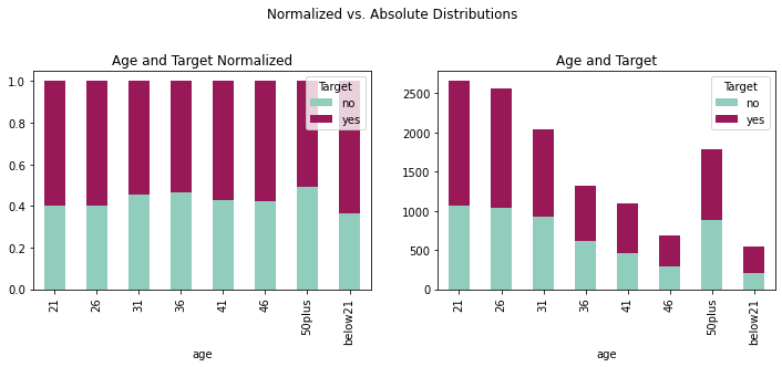
fig = plt.figure(figsize=(12,8))
ax2 = fig.add_subplot(221); ax1 = fig.add_subplot(222)
fig.suptitle('Normalized vs. Absolute Distributions')

crosstabmari = pd.crosstab(coupons_df['maritalStatus'],coupons_df['Target'])
crosstabmarinorm = crosstabmari.div(crosstabmari.sum(1), axis=0)
plotmari = crosstabmari.plot(kind='bar', stacked=True,
                             title='Marital Status and Target',
                             ax=ax1, color=['#90CDBC', '#991857'])

plotmarinorm = crosstabmarinorm.plot(kind='bar', stacked = True,
                                     title='Marital Status and Target Normalized',
                                     ax=ax2, color=['#90CDBC', '#991857'])
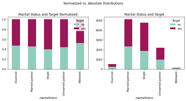
fig = plt.figure(figsize=(12,8))
ax2 = fig.add_subplot(221); ax1 = fig.add_subplot(222)
fig.suptitle('Normalized vs. Absolute Distributions')
crosstabchild = pd.crosstab(coupons_df['has_children'],
                            coupons_df['Target'])
crosstabchildnorm = crosstabchild.div(crosstabchild.sum(1), axis=0)

plotchild = crosstabchild.plot(kind='bar', stacked=True,
                               title='Child Status and Target',
                               ax=ax1, color=['#90CDBC', '#991857'])

plotchildnorm = crosstabchildnorm.plot(kind='bar', stacked=True,
                                       title='Child Status and Target Normalized',
                                       ax=ax2, color=['#90CDBC', '#991857'])
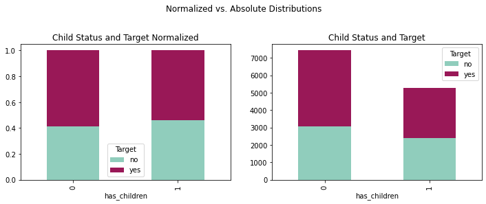
fig = plt.figure(figsize=(12,8))
ax2 = fig.add_subplot(221)
ax1 = fig.add_subplot(222)
fig.suptitle('Normalized vs. Absolute Distributions')

crosstabeduc = pd.crosstab(coupons_df['education'],coupons_df['Target'])
crosstabeducnorm = crosstabeduc.div(crosstabeduc.sum(1), axis = 0)

ploteduc = crosstabeduc.plot(kind='bar', stacked = True,
                             title = 'Education and Target',
                             ax = ax1, color = ['#90CDBC', '#991857'])


ploteducnorm = crosstabeducnorm.plot(kind='bar', stacked = True,
                                     title = 'Education and Target Normalized',
                                     ax = ax2, color = ['#90CDBC', '#991857'])
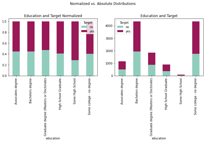
fig = plt.figure(figsize=(12,8))
ax2 = fig.add_subplot(221)
ax1 = fig.add_subplot(222)
fig.suptitle('Normalized vs. Absolute Distributions')

crosstaboccu = pd.crosstab(coupons_df['occupation'],coupons_df['Target'])
crosstaboccunorm = crosstaboccu.div(crosstaboccu.sum(1), axis = 0)

plotoccu = crosstaboccu.plot(kind='bar', stacked = True,
                             title = 'Occupation and Target',
                             ax = ax1, color = ['#90CDBC', '#991857'])


plotoccunorm = crosstaboccunorm.plot(kind='bar', stacked = True,
                                     title = 'Occupation and Target Normalized',
                                     ax = ax2, color = ['#90CDBC', '#991857'])
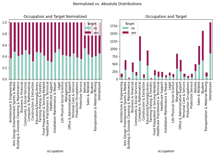
fig = plt.figure(figsize=(12,8))
ax2 = fig.add_subplot(221)
ax1 = fig.add_subplot(222)

fig.suptitle('Normalized vs. Absolute Distributions')

crosstabinco = pd.crosstab(coupons_df['income'],
                           coupons_df['Target'])

crosstabinconorm = crosstabinco.div(crosstabinco.sum(1), axis = 0)

plotinco = crosstabinco.plot(kind='bar', stacked = True,
                             title = 'Income and Target',
                             ax = ax1, color = ['#90CDBC', '#991857'])


plotinconorm = crosstabinconorm.plot(kind='bar', stacked = True,
                                     title = 'Income and Target Normalized',
                                     ax = ax2, color = ['#90CDBC', '#991857'])
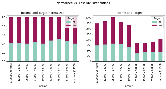
fig = plt.figure(figsize=(12, 8))
ax2 = fig.add_subplot(221)
ax1 = fig.add_subplot(222)

fig.suptitle('Normalized vs. Absolute Distributions')

crosstabcar = pd.crosstab(coupons_df['car'],coupons_df['Target'])
crosstabcarnorm = crosstabcar.div(crosstabcar.sum(1),
                                  axis = 0)

plotcar = crosstabcar.plot(kind='bar',
                           stacked=True,
                           title='Car and Target',
                           ax=ax1,
                           color=['#90CDBC', '#991857'])


plotcarnorm = crosstabcarnorm.plot(kind='bar',
                                   stacked=True,
                                   title='Car and Target Normalized',
                                   ax=ax2,
                                   color=['#90CDBC',
                                          '#991857'])
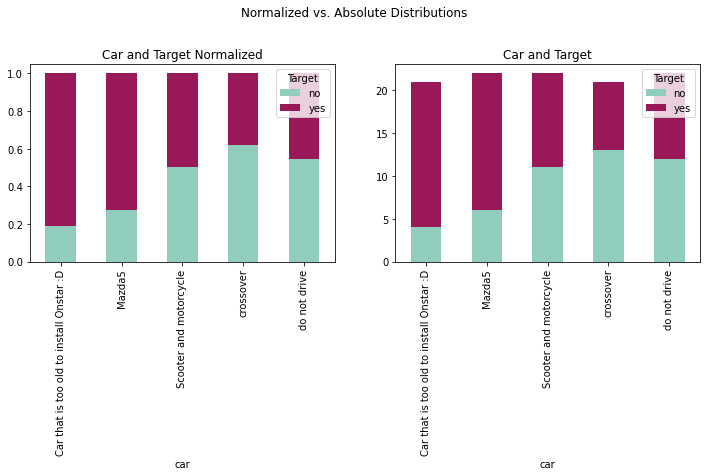
fig = plt.figure(figsize=(12,8))
ax2 = fig.add_subplot(221)
ax1 = fig.add_subplot(222)

fig.suptitle('Normalized vs. Absolute Distributions')

crosstabbar = pd.crosstab(coupons_df['Bar'], coupons_df['Target'])
crosstabbarnorm = crosstabbar.div(crosstabbar.sum(1),
                                  axis=0)

plotbar = crosstabbar.plot(kind='bar',
                           stacked=True,
                           title='Monthly Bar Visits and Target',
                           ax=ax1,
                           color=['#90CDBC',
                                  '#991857'])


plotbarnorm = crosstabbarnorm.plot(kind='bar', stacked = True,
                                   title='Monthly Bar Visits and Target ' +
                                         'Normalized',
                                   ax=ax2,
                                   color=['#90CDBC',
                                          '#991857'])
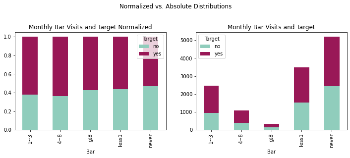
fig = plt.figure(figsize=(12,8))
ax2 = fig.add_subplot(221); ax1 = fig.add_subplot(222)
fig.suptitle('Normalized vs. Absolute Distributions')
crosstabcoff = pd.crosstab(coupons_df['CoffeeHouse'], coupons_df['Target'])
crosstabcoffnorm = crosstabcoff.div(crosstabcoff.sum(1), axis = 0)
plotcoff = crosstabcoff.plot(kind='bar', stacked=True,
                             title='Monthly Coffee House Visits and Target',
                             ax=ax1, color=['#90CDBC', '#991857'])
plotcoffnorm = crosstabcoffnorm.plot(kind='bar', stacked=True,
title = 'Monthly Coffee House Visits and Target Normalized',
                                     ax=ax2, color=['#90CDBC', '#991857'])
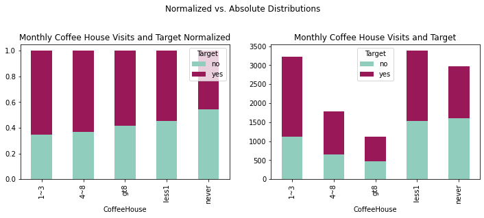
fig = plt.figure(figsize=(12,8))
ax2 = fig.add_subplot(221)
ax1 = fig.add_subplot(222)
fig.suptitle('Normalized vs. Absolute Distributions')

crosstabcarr = pd.crosstab(coupons_df['CarryAway'],coupons_df['Target'])
crosstabcarrnorm = crosstabcarr.div(crosstabcarr.sum(1), axis = 0)

plotcarr = crosstabcarr.plot(kind='bar', stacked = True,
                             title = 'Monthly Carry Away Visits and Target',
                             ax = ax1, color = ['#90CDBC', '#991857'])

plotcarrnorm = crosstabcarrnorm.plot(kind='bar', stacked = True,
title = 'Monthly Carry Away Visits and Target Normalized',
                                     ax = ax2, color = ['#90CDBC', '#991857'])
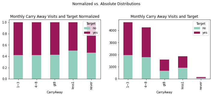
fig = plt.figure(figsize=(14,8))
ax2 = fig.add_subplot(221)
ax1 = fig.add_subplot(222)
fig.suptitle('Normalized vs. Absolute Distributions')

crosstabLess = pd.crosstab(coupons_df['RestaurantLessThan20'],coupons_df['Target'])
crosstabLessnorm = crosstabLess.div(crosstabLess.sum(1), axis = 0)

plotLess = crosstabLess.plot(kind='bar', stacked = True,
title = 'Restaurant Visits a Month Less than $20/person and Target',
                             ax = ax1, color = ['#90CDBC', '#991857'])

plotLessnorm = crosstabLessnorm.plot(kind='bar', stacked = True,
title = 'Restaurant Visits a Month Less than $20/person and Target Normalized',
                                     ax = ax2, color = ['#90CDBC', '#991857'])
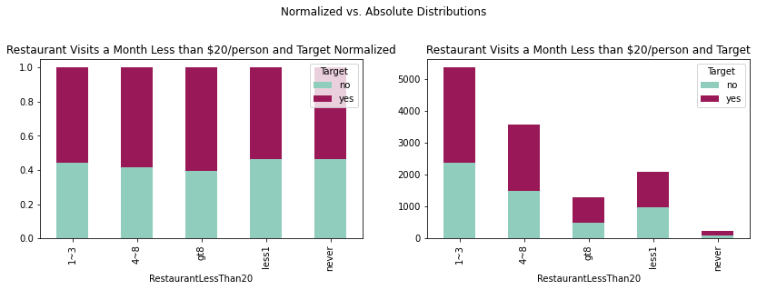
fig = plt.figure(figsize=(14,8))
ax2 = fig.add_subplot(221)
ax1 = fig.add_subplot(222)
fig.suptitle('Normalized vs. Absolute Distributions')

crosstabTo50 = pd.crosstab(coupons_df['Restaurant20To50'],coupons_df['Target'])
crosstabTo50norm = crosstabTo50.div(crosstabTo50.sum(1), axis = 0)

plotTo50 = crosstabTo50.plot(kind='bar', stacked = True,
title = 'Restaurant Visits a Month $20-50/person and Target',
                             ax = ax1, color = ['#90CDBC', '#991857'])

plotTo50norm = crosstabTo50norm.plot(kind='bar', stacked = True,
title = 'Restaurant Visits a Month $20-50/person and Target Normalized',
                                     ax = ax2, color = ['#90CDBC', '#991857'])
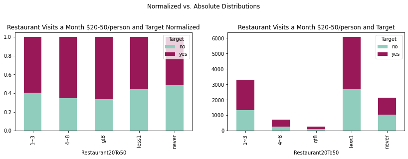
fig = plt.figure(figsize=(14,8))
ax2 = fig.add_subplot(221)
ax1 = fig.add_subplot(222)
fig.suptitle('Normalized vs. Absolute Distributions')

crosstab5min = pd.crosstab(coupons_df['toCoupon_GEQ5min'],coupons_df['Target'])
crosstab5minnorm = crosstab5min.div(crosstab5min.sum(1), axis = 0)

plot5min = crosstab5min.plot(kind='bar', stacked = True,
                             title = 'Coupon over 5 min away and Target',
                             ax = ax1, color = ['#90CDBC', '#991857'])


plot5minnorm = crosstab5minnorm.plot(kind='bar', stacked = True,
title = 'Coupon over 5 min away and Target Normalized',
                             ax = ax2, color = ['#90CDBC', '#991857'])
fig = plt.figure(figsize=(14,8))
ax2 = fig.add_subplot(221)
ax1 = fig.add_subplot(222)
fig.suptitle('Normalized vs. Absolute Distributions')

crosstab15min = pd.crosstab(coupons_df['toCoupon_GEQ15min'],
                            coupons_df['Target'])
crosstab15minnorm = crosstab15min.div(crosstab15min.sum(1),
                                      axis = 0)

plot15min = crosstab15min.plot(kind='bar',
                               stacked = True,
title = 'Coupon over 15 min away and Target',
                               ax = ax1,
                               color = ['#90CDBC', '#991857'])

plot15minnorm = crosstab15minnorm.plot(kind='bar',
                                       stacked = True,
title = 'Coupon over 15 min away and Target Normalized',
                                       ax = ax2,
                                       color = ['#90CDBC', '#991857'])
fig = plt.figure(figsize=(14,8))
ax2 = fig.add_subplot(221)
ax1 = fig.add_subplot(222)
fig.suptitle('Normalized vs. Absolute Distributions')

crosstab25min = pd.crosstab(coupons_df['toCoupon_GEQ25min'],coupons_df['Target'])
crosstab25minnorm = crosstab25min.div(crosstab25min.sum(1), axis = 0)

plot25min = crosstab25min.plot(kind='bar', stacked = True,
title = 'Coupon over 25 min away and Target',
                               ax = ax1, color = ['#90CDBC', '#991857'])


plot25minnorm = crosstab25minnorm.plot(kind='bar', stacked = True,
title = 'Coupon over 25 min away and Target Normalized',
                                       ax = ax2, color = ['#90CDBC', '#991857'])
fig = plt.figure(figsize=(14,8))
ax2 = fig.add_subplot(221)
ax1 = fig.add_subplot(222)

fig.suptitle('Normalized vs. Absolute Distributions')

crosstabsame = pd.crosstab(coupons_df['direction_same'],
                           coupons_df['Target'])
crosstabsamenorm = crosstabsame.div(crosstabsame.sum(1),
                                    axis = 0)

plotsame = crosstabsame.plot(kind='bar',
                             stacked = True,
title = 'Coupon Same Direction and Target',
                             ax = ax1,
                             color = ['#90CDBC', '#991857'])

plotsamenorm = crosstabsamenorm.plot(kind='bar',
                                     stacked = True,
title = 'Coupon Same Direction and Target Normalized',
                                     ax = ax2,
                                     color = ['#90CDBC', '#991857'])
fig = plt.figure(figsize=(14,8))
ax2 = fig.add_subplot(221)
ax1 = fig.add_subplot(222)
fig.suptitle('Normalized vs. Absolute Distributions')
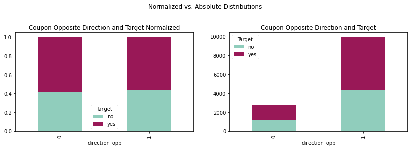
crosstabopp = pd.crosstab(coupons_df['direction_opp'],coupons_df['Target'])
crosstaboppnorm = crosstabopp.div(crosstabopp.sum(1), axis = 0)
plotopp = crosstabopp.plot(kind='bar', stacked = True,
title = 'Coupon Opposite Direction and Target',
ax = ax1, color = ['#90CDBC', '#991857'])
plotoppnorm = crosstaboppnorm.plot(kind='bar', stacked = True,
title = 'Coupon Opposite Direction and Target Normalized',
ax = ax2, color = ['#90CDBC', '#991857'])
Dropping Unnecessary Columns
With a 99.15% missing percentage, any imputation method would be impractical and the variable car will be dropped
Since 'toCoupon_GEQ5min Column' is a constant feature, we remove it.
Since 'direction_opp' is a highly correlated variable, it is dropped as well.
coupons_df.drop(columns=['car'], inplace=True)
coupons_df.drop(columns=['toCoupon_GEQ5min'], inplace=True)
coupons_df.drop(columns=['direction_opp'], inplace=True)
Examining Correlations
corr = coupons_df.corr()
corr.style.background_gradient(cmap='coolwarm')
Evaluation of Imputation Methods
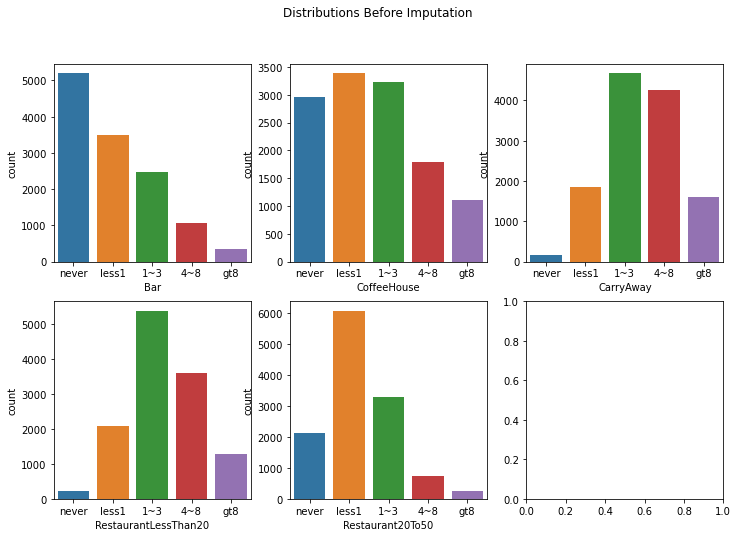
The variables Bar, CoffeeHouse, CarryAway, RestaurantLessThan20, Restaurant20To50, have a low null count $ < 2\%$. We will evaluate different imputation methods that best preserves the distribution of the data.
fig, axes = plt.subplots(2, 3, figsize=(12, 8))

likert_vals = ['never', 'less1', '1~3', '4~8', 'gt8']

fig.suptitle('Distributions Before Imputation')
sns.countplot(ax=axes[0, 0], data=coupons_df,
              x="Bar", order=likert_vals)
sns.countplot(ax=axes[0, 1], data=coupons_df,
              x="CoffeeHouse", order=likert_vals)
sns.countplot(ax=axes[0, 2], data=coupons_df,
              x="CarryAway", order=likert_vals)
sns.countplot(ax=axes[1, 0], data=coupons_df,
              x="RestaurantLessThan20", order=likert_vals)
sns.countplot(ax=axes[1, 1], data=coupons_df,
              x="Restaurant20To50", order=likert_vals)
plt.show()
KL Divergence
The Kullback-Leibler Divergence will be used to determine the amount the distribution of each variable diverges after imputation. The imputation method with the smallest KL divergence will be selected.
def kl_divergence(p, q):
    return sum(p * np.log(p/q))
Imputation Methods
- Median Imputation
- Frequent Imputation
The values of the variables Bar, CoffeeHouse, CarryAway, RestaurantLessThan20, Restaurant20To50, appear to be values from a likert scale. These are ordinal values, so they will be converted accordingly, before median imputation can be used.
impute_test = coupons_df[['Bar', 'CoffeeHouse', 'CarryAway',
                         'RestaurantLessThan20', 'Restaurant20To50']]
impute_test.replace({'never': 0, 'less1': 1, '1~3': 2, '4~8': 3, 'gt8': 4},
                    inplace=True)
# Store KL results
cols = ['Bar', 'CoffeeHouse', 'CarryAway', 'RestaurantLessThan20',
        'Restaurant20To50']
kl_results = pd.DataFrame(index=cols)
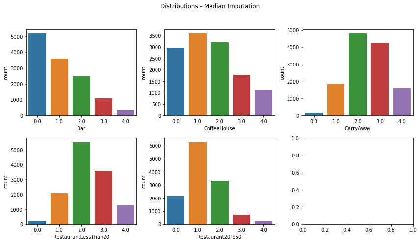
Median Imputation
med_impute = SimpleImputer(missing_values=np.nan, strategy='median')
med_impute_df = pd.DataFrame(med_impute.fit_transform(impute_test),
                             columns=['Bar', 'CoffeeHouse', 'CarryAway',
                                      'RestaurantLessThan20', 'Restaurant20To50'])
fig, axes = plt.subplots(2, 3, figsize=(12, 7))
fig.suptitle('Distributions - Median Imputation')
sns.countplot(ax=axes[0, 0], data=med_impute_df, x="Bar")
sns.countplot(ax=axes[0, 1], data=med_impute_df, x="CoffeeHouse")
sns.countplot(ax=axes[0, 2], data=med_impute_df, x="CarryAway")
sns.countplot(ax=axes[1, 0], data=med_impute_df, x="RestaurantLessThan20")
sns.countplot(ax=axes[1, 1], data=med_impute_df, x="Restaurant20To50")
plt.tight_layout(rect=[0, 0, 1, 0.9]); plt.show()
med_results = []
for col in cols:
    p = impute_test[col].dropna()
    p = p.groupby(p).count() / p.shape[0]
    q = med_impute_df[col].groupby(med_impute_df[col]).count() / \
      med_impute_df[col].shape[0]

    print('P(%s = x) = %s' % (col, p.to_list()))
    print('Q(%s = x) = %s' % (col, q.to_list()))
    print('KL Divergence: %f' % kl_divergence(p, q))
    print('\n')
    med_results.append(kl_divergence(p, q))
kl_results['Median Imputation'] = med_results
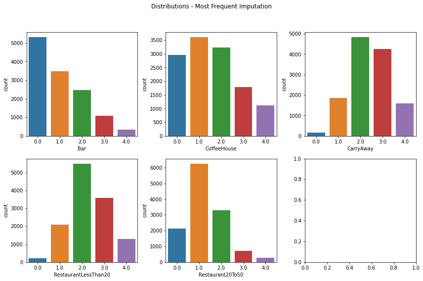
Frequent Imputation
freq_impute = SimpleImputer(missing_values=np.nan, strategy='most_frequent')
freq_impute_df = pd.DataFrame(freq_impute.fit_transform(impute_test),
                              columns=['Bar', 'CoffeeHouse', 'CarryAway',
                                       'RestaurantLessThan20', 'Restaurant20To50'])
fig, axes = plt.subplots(2, 3, figsize=(12, 8))

fig.suptitle('Distributions - Most Frequent Imputation')
sns.countplot(ax=axes[0, 0], data=freq_impute_df, x="Bar")
sns.countplot(ax=axes[0, 1], data=freq_impute_df, x="CoffeeHouse")
sns.countplot(ax=axes[0, 2], data=freq_impute_df, x="CarryAway")
sns.countplot(ax=axes[1, 0], data=freq_impute_df, x="RestaurantLessThan20")
sns.countplot(ax=axes[1, 1], data=freq_impute_df, x="Restaurant20To50")
plt.tight_layout(rect=[0, 0, 1, 0.9]); plt.show()
freq_results = []
for col in cols:
    p = impute_test[col].dropna()
    p = p.groupby(p).count() / p.shape[0]
    q = freq_impute_df[col].groupby(freq_impute_df[col]).count() / \
    freq_impute_df[col].shape[0]

    print('P(%s = x) = %s' % (col, p.to_list()))
    print('Q(%s = x) = %s' % (col, q.to_list()))
    print('KL Divergence: %f' % kl_divergence(p, q))
    print('\n')
    freq_results.append(kl_divergence(p, q))
kl_results['Frequent Imputation'] = freq_results
KL Divergence of Imputation Methods
kl_results
As shown in the table above, the imputation methods are almost identical with Imputation by Most Frequent Value (Mode) having a slightly lower KL Divergence for the variable Bar. Imputation by Most Frequent Value will be used.
Imputation by Most Frequent Value
# replace values of Bar, CoffeeHouse, CarryAway,
# RestaurantLessThan20, Restaurant20To50 as ordinal
coupons_df[cols] = coupons_df[cols].replace({'never': 0,
                                             'less1': 1, '1~3': 2,
                                             '4~8': 3, 'gt8': 4})
coupons_df[cols] = SimpleImputer(missing_values=np.nan,
                   strategy='most_frequent').fit_transform(coupons_df[cols])
null_vals = pd.DataFrame(coupons_df.isna().sum(), columns=['Null Count'])
null_vals['Null Percent'] = (null_vals['Null Count'] / coupons_df.shape[0]) * 100
null_vals
Preprocessing
coupons_df = pd.read_csv('https://archive.ics.uci.edu/ml/\
machine-learning-databases/00603/in-vehicle-coupon-recommendation.csv')
coupons_df.head()
# define columns types
nom = ['destination', 'passenger', 'weather', 'coupon',
       'gender', 'maritalStatus', 'occupation']
bin = ['gender', 'has_children', 'toCoupon_GEQ15min',
       'toCoupon_GEQ25min', 'direction_same']
ord = ['temperature', 'age', 'education', 'income',
       'Bar', 'CoffeeHouse', 'CarryAway', 'RestaurantLessThan20',
       'Restaurant20To50']
num = ['time', 'expiration']
ex = ['car', 'toCoupon_GEQ5min', 'direction_opp']
# Convert time to 24h military time
def convert_time(x):
    if x[-2:] == "AM":
        return int(x[0:-2]) % 12
    else:
        return (int(x[0:-2]) % 12) + 12

def average_income(x):
    inc = np.array(x).astype(np.float)
    return sum(inc) / len(inc)

def pre_process(df):
    # keep original dataframe imutable
    ret = df.copy()

    # Drop columns
    ret.drop(columns=['car', 'toCoupon_GEQ5min', 'direction_opp'],
             inplace=True)

    # rename values
    ret = ret.rename(columns={'passanger':'passenger'})
    ret['time'] = ret['time'].apply(convert_time)
    ret['expiration'] = ret['expiration'].map({'1d':24, '2h':2})

    # convert the following columns to ordinal values
    ord_cols = ['Bar', 'CoffeeHouse', 'CarryAway', 'RestaurantLessThan20',
                'Restaurant20To50']
    ret[ord_cols] = ret[ord_cols].replace({'never': 0, 'less1': 1,
                                                 '1~3': 2, '4~8': 3, 'gt8': 4})

    # impute missing
    ret[ord_cols] = SimpleImputer(missing_values=np.nan,
                       strategy='most_frequent').fit_transform(ret[ord_cols])

    # Changing coupon expiration to uniform # of hours
    ret['expiration'] = coupons_df['expiration'].map({'1d':24, '2h':2})

    # Age, Education, Income as ordinal
    ret['age'] = ret['age'].map({'below21':1,
                                                 '21':2,'26':3,
                                                 '31':4,'36':5,
                                                 '41':6,'46':6,
                                                 '50plus':7})
    ret['education'] = ret['education'].map(\
                            {'Some High School':1,
                             'Some college - no degree':2,
                             'Bachelors degree':3, 'Associates degree':4,
                             'High School Graduate':5,
                             'Graduate degree (Masters or Doctorate)':6})
    ret['average income'] = ret['income'].str.findall('(\d+)').apply(average_income)
    ret['income'].replace({'Less than $12500': 1, '$12500 - $24999': 2,
                           '$25000 - $37499': 3, '$37500 - $49999': 4,
                           '$50000 - $62499': 5, '$62500 - $74999': 6,
                           '$75000 - $87499': 7, '$87500 - $99999': 8,
                           '$100000 or More': 9}, inplace=True)

    # Change gender to binary value
    ret['gender'].replace({'Male': 0, 'Female': 1}, inplace=True)

    # One Hot Encode
    nom = ['destination', 'passenger', 'weather', 'coupon',
           'maritalStatus', 'occupation']
    for col in nom:
        # k-1 cols from k values
        ohe_cols = pd.get_dummies(ret[col], prefix=col, drop_first=True)
        ret = pd.concat([ret, ohe_cols], axis=1)
        ret.drop(columns=[col], inplace=True)

    return ret
# Simple function to prep a dataframe for a model
def scale_data(df, std, norm, pass_cols):
    """
    df: raw dataframe you want to process
    std: list of column names you want to standardize (0 mean unit variance)
    norm: list of column names you want to normalize (min-max)
    pass_cols: list of columns that do not require processing (target var, etc.)

    returns: prepped dataframe
    """
    ret = df.copy()
    # Only include columns from lists
    ret = ret[std + norm + pass_cols]
    # Standardize scaling for gaussian features
    if (isinstance(std, list)) and (len(std) > 0):
        ret[std] = StandardScaler().fit(ret[std]).transform(ret[std])
    # Normalize (min-max) [0,1] for non-gaussian features
    if (isinstance(norm, list)) and (len(norm) > 0):
        ret[norm] = Normalizer().fit(ret[norm]).transform(ret[norm])


    return ret
# Processed data (remove labels from dataset)
coupons_proc = pre_process(coupons_df.drop(columns='Y'))

# Labels
labels = coupons_df['Y']

# Standardize/Normalize
to_scale = ['average income', 'temperature', 'time', 'expiration']
coupons_proc = scale_data(coupons_proc, to_scale, [],
list(set(coupons_proc.columns.tolist()).difference(set(to_scale))))

coupons_proc.head()
coupons_df
Selecting Predictors for Modeling
X = pd.DataFrame(coupons_proc[['average income', 'education', 'expiration',
                             'age','temperature','has_children']])
Generalized Linear Model
Logistic Regression
Link Function for Binary Response
$$ X\beta = \text{ln} \frac{\mu}{1-\mu} $$where $e^{\text{ln}(x)}=x$ and,
$$ \mu = \frac{e^{X\beta}}{1+e^{X\beta}} $$Logistic Regression - Parametric Form
Logistic Regression - Descriptive Form
X = sm.add_constant(X)
y = pd.DataFrame(coupons_df[['Y']])
X_train, X_test, y_train, y_test = train_test_split(X, y,
                                   test_size=0.20, random_state=42)
log_results = sm.Logit(y_train, X_train).fit()
log_results.summary()
Whether or not an individual has children bears no statistical significance for this baseline model at a p-value of 0.107. Thus, we omit this predictor from this model.
That being said, we will explore re-introducing these for subsequent models
X = pd.DataFrame(coupons_proc[['average income', 'education', 'expiration',
                               'temperature','has_children']])
The refined logistic regression equation becomes:
$\small{\hat{p}(\text{coupons}) = \frac{\text{exp}(0.0147-0.000001821(\text{average income})-0.0512(\text{education})+0.0262(\text{expiration})-0.0053(\text{age})+0.0079(\text{temperature}))}{1+\text{exp}(0.0147-0.000001821(\text{average income})-0.0512(\text{education})+0.0262(\text{expiration})-0.0053(\text{age})+0.0079(\text{temperature}))}}$
logreg = LogisticRegression()
logreg.fit(X_train, y_train)
y_pred = logreg.predict(X_test)
pred_log = [round(num) for num in y_pred]
confusion_matrix(y_test, pred_log)
plot_confusion_matrix(logreg, X_test, y_test)
plt.title('Confusion Matrix - Logistic Regression')
plt.show()
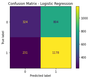
print(classification_report(y_test, y_pred))
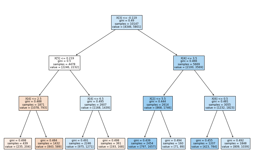
Decision Tree Classifier
coupon_tree = tree.DecisionTreeClassifier(max_depth=3)
coupon_tree = coupon_tree.fit(X_train,y_train)

y_pred = coupon_tree.predict(X_test)

print('accuracy %2.2f ' % accuracy_score(y_test,y_pred))
print(classification_report(y_test, y_pred))
fig, ax = plt.subplots(figsize = (15, 10))
short_treeplot = tree.plot_tree(coupon_tree, filled=True)
plt.tight_layout(rect=[0, 0, 0, 0])
plt.show()