Identifying Safer Pedestrian Routes in Los Angeles
Leonid Shpaner, Christopher Robinson, and Jose Luis Estrada
| Python Code | Description |
|---|---|
| Python - Compiled Jupyter Notebook | This notebook contains the primary code base for the data science portions of the project, consisting of Data Exploration Phase I, Data Preparation, Data Exploration Phase II, and Modeling. |
| Data Exploration Phase I | This notebook provides a data report mapping to unique ID fields, column names, data types, null counts, and percentages in the dataframe. It also shows some basic bar graphs for an initial cursory overview of data exploration. |
| Data Preparation | This notebook preprocesses the dataframe, allowing for further exploration to take place and sets the stage for modeling. |
| Data Exploration Phase II | This notebook takes a more granular look into the columns of interest using boxplots, stacked bar graphs, histograms, and culminates with a correlation matrix. |
| Modeling | This notebook contains all of the machine learning algorithms carried out in this project. |
| Functions |
This .py file creates functions for data types and various plots that are used throughout the project pipeline.
|
ABSTRACT
An increasing number of environmentally conscious individuals are using various forms of pedestrian travel in large cities around the United States. Due to the recent increase in violent crime, it is crucial to be aware of safety when navigating through unfamiliar areas. The goal of this project was to use data science techniques to create an application to help individuals navigate unfamiliar areas safely. A data pipeline was created, utilizing Python and GIS, to download and process Los Angeles Police Department crime data for use in predictive modeling. Various models were created and tested; however, XGBoost outperformed all other models based on accuracy, precision, recall, and f1-score. The model output was configured in a GIS web application which used crime predictions and historical data to determine the safest route between locations. The results for both the model and the GIS routing application have been positive. The model performed well on the test data; however, the model outcomes alone are likely not sufficient for ensuring safety. Additional information could add insight and further research may be necessary to determine the most important considerations for pedestrian safety.
KEYWORDS
Crime, Safety, GIS, Machine Learning.
1 Introduction
Forms of environmentally friendly travel, such as walking, biking, and public transportation, are often used in large cities by environmentally conscious individuals. Unfortunately, pedestrian travel leaves people more exposed to violence in high crime areas. Currently, violent crime in large cities is on the rise and law enforcement is understaffed. The best way to protect yourself from violence is to avoid it altogether. However, it can be difficult to avoid high crime areas, especially in our quickly changing social environment.
2 Background
Murders have spiked nearly 40% since 2019, and violent crimes, including shootings and assaults, have increased overall (Bura et al., 2019). Violent crimes comprise four offenses — murder or nonnegligent manslaughter, rape, robbery, and aggravated assault. Pedestrian travel, whether for recreation or necessity, is part of everyday life for millions of urban Americans, and safety is a growing concern. Many people feel that because they are local to an area, they are fully aware of the risks associated with traveling around the area. In a large densely populated area, such as Los Angeles, California, it can be difficult even for locals to be well informed of the safety relative to all the communities which surround them. Additionally, with social and political unrest due to situations like the George Floyd killing and the supreme court decision regarding Roe v. Wade, safety, especially in urban communities, can change rapidly.
2.1 Problem Identification and Motivation
Due to increases in violent crime and constantly evolving social environments, it is crucial to understand the level of safety when navigating through different areas. Unfortunately, this requires an intimate knowledge of the area or significant research by the navigator. It is imperative to public safety to provide simple solutions to increase safety when traveling between locations. Whether for leisure or necessity, travel is an essential part of life. People are especially vulnerable when traveling to new areas; however, in today’s quickly changing social environment, even local travel has been affected by the surge in violent crime. Knowing how safe you are in a specific area can be challenging. Even with access to crime data, it can be difficult to understand what information is relevant and may involve a thorough investigation which could be overwhelming for some individuals. Students are especially aware of the challenges to safety while traveling locally as many students often use alternative forms of transportation to and from school, and colleges, such as the University of California, are near high crime areas.
2.2 Definition of Objectives
This project examines pedestrian safety using machine learning and recent crime data. The goal is to automate a process to identify the safest route between locations, as well as provide additional up to date crime information. This project is looking for the “safest” route, which does not guarantee the route is safe. In some instances, there is no “safe” route. Additionally, where crime is concerned, often factors such as time of day and traits relating to the victim such as age, sex, and race, are elements of safety. The solution discussed here not only identifies the safest route but includes elements of situational awareness to assist in making the best decision possible regarding personal safety. When it comes to navigating an area safely, recommendations can be made, but ultimately it is up to the navigator to determine what level of risk is acceptable.
3 Literature Review
There are other studies relating to safety and routing using crime reporting, density mapping, distance, and various methods of machine learning. While efficient routing through high crime areas is the primary goal, it is important to realize that sometimes there is no safe route through an area. In these cases, routing only provides partial information and other data are required to make an informed decision. Past research has often focused on specific groups, such as women. With the changing trends in crime, such as increasing assaults on Asian Americans and the elderly, it has become increasingly important to be more inclusive when deciding what factors are important regarding safety and who may be most at risk in each area.
3.2 Predicting Secure and Safe Route for Women using Google Maps
Solutions, in general, recommend the safest route between locations, but different groups can be affected by crime in various ways. Women can encounter more challenges than men, and different parameters need to be taken into consideration to provide the safest route for women. This solution offers techniques utilizing Google Maps technology to identify the safest route for women (Lopez, 2022).
3.3 Applying Google Maps and Google Street View in Criminological Research
There is growing concern that cost-effective web-based mapping applications such as Google Maps and Google Street View could be exploited by criminals, such as graffiti artists, shoplifters, and terrorists to plan criminal activity more effectively. Alternatively, there is the potential to use these applications to expand on criminology research, given that the number of studies is still limited. This research discusses how online mapping applications can identify new research questions and methodological additions to criminology (Vandeviver, 2014).
3.4 Algorithm to Determine the Safest Route
The Iterative Dichotomiser 3 (ID3) decision tree algorithm is proposed to classify safety risk based on streets and their corresponding routes in San Francisco with 12 years of data given that crime has been on the rise (Tarkelar et al., 2016); the goal is to iterate through a list of all streets to determine whether the route is safe or not (binary outcome). Proposing the usage of the ID3 decision classifier is not a sound and proper methodology because not all features are nominal. Hence, reproducibility must be accommodated, and therefore, most machine learning algorithms use numerical datatypes without the challenge of calculating information entropy (Wang et al., 2017).
3.5 Envision of Route Safety Direction Using Machine Learning
Predicting the safety of women in Delhi is an important step in advancing multidisciplinary and multi-faceted socioeconomic research regarding women’s contribution to society. The proposed k-means clustering algorithm uses 1481 records to train and 634 records to test with an accuracy score of only 79.7%. The model can benefit from additional performance metrics like f1-score, recall, and precision in conjunction with subsequent retraining an additional validation holdout set, or at least a five k-fold cross-validation (Pavate et al., 2019).
4 Methodology
An automated data pipeline was created using the Python programming language (version 3.7.13) to download and preprocess the source data prior to modeling. The datasets were merged using a combination of Python and ArcGIS (version 10.8) and the resulting output was exported for subsequent exploratory data analysis and further preprocessing. The resulting data contains 183,362 rows and 80 columns. Figure 1 outlines the project workflow.
4.1 Data Acquisition and Aggregation
The dataset was downloaded from the Los Angeles Police Department (LAPD, 2022) and preprocessed using the ArcGIS ArcPy library. Each crime data point was spatially joined to street segments within 50 feet, producing a one-to-many relationship between streets and crimes.
Figure 1
Project Workflow

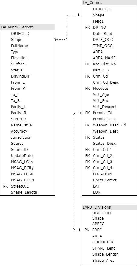
The resulting dataset contained merged street and crime data. The merged dataset was then joined to Los Angeles police districts to extract the district description. This was done to validate the existing district field in the Los Angeles Police Department crime data. The join added district descriptions to streets where the descriptions were null because they did not have crimes associated with them. Once all three datasets were joined, all records with null street ID values were dropped and the dataset was exported to .csv for exploratory data analysis and further preprocessing. Figure 2 outlines the architecture for the datasets.
Figure 2
Data Architecture
4.1.1. Exploratory Data Analysis. The top three ages of crime victims are 25-30, 20-25, and 30-35, with ages 25-30 reporting 25,792 crimes, ages 20-25 reporting 22,235 crimes, and ages 30-35 reporting 21,801 crimes, respectively. The average age of male victims is approximately 36 years old (see Table 1), whereas the mean age of female victims is approximately 34 years old.
Table 1
Sex Summary Statistics by Age
|
Sex |
Mean |
Median |
SD |
Min |
Max |
|---|---|---|---|---|---|
|
F |
34.4 |
32 |
15.2 |
0 |
99 |
|
M |
36.3 |
35 |
16.5 |
0 |
99 |
|
X |
5.69 |
0 |
13 |
0 |
120 |
Note. Unknown sexes show a mean age of approximately six years old and a median of zero (newborns or infants). The mean age values are greater than the median age values which corresponds to a positively skewed distribution. The unknown sex shows the lowest mean, but the highest maximum age which also creates a positive skew.
Crime severity occurs at almost an even rate by age group, except for the highest age range of 115-120, where crime incidence is lower, but overall, more serious. Moreover, there are 19,073 more serious crimes than less serious crimes, comprising a majority (55.56%) of all cases. Crimes tend to be less severe in pedestrian walkways, paved or unpaved private roads, and trails when compared to primary roads, minor roads, and alleys.
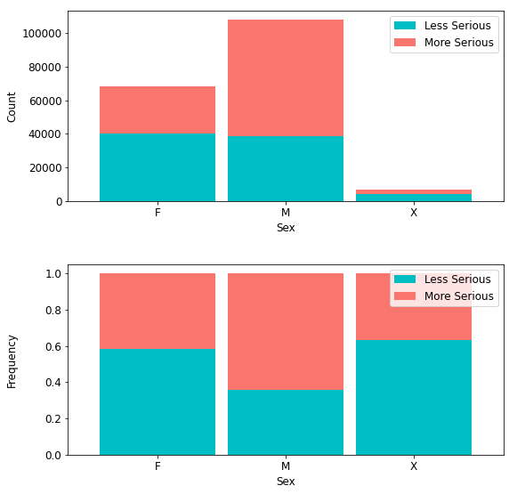
4.1.1.1. Crime Severity by Sex. The male population is larger than the female population in this dataset, Table 2 shows from both the regular and normalized distributions, respectively, that more serious crimes occur with a higher prevalence (69,370) for males than females (28,565). This corresponds to 64.24% of more serious crimes occurring for males and 41.70% occurring for females. Although, for unknown sexes, there exists a 36.70% prevalence rate for more serious crimes. Whenever crime exists in the unknown demographic it occurs with less prevalence and less seriousness for males than females.
Table 2
Crime Severity by Sex
|
Sex |
Less |
More |
Total |
% Severe |
|---|---|---|---|---|
|
F |
39,936 |
28,565 |
68,501 |
42 |
|
M |
38,615 |
69,370 |
107,985 |
64 |
|
X |
4,219 |
2,446 |
6,665 |
37 |
|
Total |
82,770 |
100,381 |
183,151 |
55 |
Figure 3 shows absolute and normalized bar graphs of crime severity by sex.
Figure 3
Crime Severity by Sex
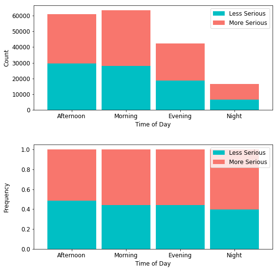
4.1.1.3. Crime Severity by Time of Day. Figure 4 shows that more serious crimes (35,396) occur in the morning than any other time of day. Evening crimes are generally more serious, but account for less crimes in total than those in the morning or afternoon. More serious night crimes account for only 9,814 (approximately 10%) of all such crimes. However, 60% of crimes occurring at night are more serious and crimes in the afternoon give no preference to severity, occurring at about equal rates.
Figure 4
Crime Severity by Time of Day
4.1.1.4. Crime Severity by Month. The month of June presents a record of 10,852 more serious crimes than any other month, so there exists a higher prevalence of more serious crimes mid-year than any other time of year.
4.1.1.5. Crime Severity by Descent. In terms of descent, members of the Hispanic/Latin/Mexican demographic account for 51,601 incidences of more serious crimes. More importantly, Table 3 illustrates that with an additional 40,226 less serious crimes, this demographic accounts for a total of 91,827 crimes (50% of all crimes in the data).
4.1.1.6. Crime Severity by Neighborhood. The 77th Street region shows the highest amount of more serious crimes (14,350), more than any other district; second is the Southeast area (10,142). It is equally important to note that most crimes (100,487 or ~55%) occur on the street, with 57.5% being attributed to more serious crimes.
4.2 Data Quality
The preprocessing stage began by inspecting each column’s data types for null values.
4.2.1. There were 3,274 missing values for weapon description. Imputation was necessary to properly assign the corresponding numerical value to the corresponding weapons used code, which was also missing 3,274 observations.
4.2.1.1. Victim Descent. The victim descent column had 171 missing values; the rows corresponding to these values were imputed with “unknown” rather than dropped since descent here remains unknown.
4.2.1.2. Victim’s Sex. The same holds true for victim’s sex, where there were 167 missing values. Descent and age are important features which were numericized and adapted for use with machine learning. All string columns were omitted from the development (modeling) set.
4.2.1.3. Weapons Used. The weapons used column contains useful information, and the rows of missing data presented therein were imputed by a value of 500, corresponding to “unknown” in the data dictionary. Similarly, the missing values in victim’s sex and descent, respectively, were imputed by a categorical value of “X,” for “unknown.” The 211 missing values contained in the zip code column were dropped since they could not be logically imputed.
4.3 Feature Engineering
Certain columns presented in their raw form were not adaptable to a binary classification task within a machine learning algorithm. For example, columns containing object data types that are useful for analysis could be numerically encoded into new columns that could provide this information more appropriately. There existed two date columns (date reported and date occurred) of which only the latter was used for extracting the year and month into two new columns, respectively, since a date object input feature may not be useful in a machine learning algorithm. In addition, descriptions of street premises were first converted into lower case strings within the column and subsequently encoded into separate binarized columns. Similarly, new columns for time (derived from military time) and city neighborhoods (derived from area) were encoded into binarized columns, respectively.
4.3.1 Reclassifying Useful Categorical Features. Sex and descent are critical factors in making informed decisions about crime. New columns were created for both variables to better represent their characteristics. For example, unidentified sexes were replaced with unknown, and one-letter abbreviations for victim descent were re-categorized by full-text descent descriptions from the city of Los Angeles’ data dictionary.
4.3.1.1. Exclusion Criteria. Any columns with all null rows and object data types were immediately dropped from the dataset but cast into a new dataframe for posterity. Furthermore, only data from the year 2022 was included, because older retrospective data does not represent an accurate enough depiction of crime in the city of Los Angeles. Longitude and latitude columns were dropped because city neighborhood columns took their place for geographic information. Moreover, columns from previous joins, identifications, report numbers, and categorical information encoded to the original dataframe were omitted from this dataframe. Columns that only present one unique value (Pedestrian Overcrossing and Tunnel) were removed. Lastly, any column (military time) that presented over and above the Pearson correlation threshold of r = 0.75 was dropped to avoid between-predictor collinearity; all numeric values in the dataframe were cast to integer type formatting. Data types were examined once more on this preprocessed dataset to ensure that all data types were integers, and no columns remained null. At this stage, there were 42,072 rows and 38 columns.
4.4 Modeling
Certain algorithms are better adapted for delineating between violent and non-violent crimes. Tree-based classifiers performed better on crime data when identifying the safest route between locations. Outcome is based on predicted probabilities of the top performing model.
4.4.1 Selection of modeling techniques. Various models were chosen based on the assumptions as to how each model would perform. For example, certain models served as baseline predictors and did not require hyperparameter tuning.
4.4.1.1. Training, Validation, and Test Partitioned Datasets. The data were split into a 50% training (21,036 rows) and 50% holdout sets, where validation and test sets each had 10,518 rows. Three separate files were saved to the data folder path.
4.4.1.2. Quadratic Discriminant Analysis. A form of nonlinear discriminant analysis (quadratic discriminant analysis) was used with an assumption that the data followed a Gaussian distribution such that a “class-specific covariance structure can be accommodated” (Kuhn & Johnson, 2016, p. 330). This method was used to improve performance over a standard linear discriminant analysis (LDA) whereby the class boundaries are linearly separable. It does not require hyperparameters because it has a closed-form solution (Pedregosa et al., 2011).
4.4.1.4. Logistic Regression. Logistic regression was deployed next for its ability to handle binary classification tasks with relative ease. The generalized linear model takes the following form:
\[ y = \beta_0 + \beta_1x_1 +\beta_2x_2 +\cdots+\beta_px_p + \varepsilon \]
Describing the relationship between several important coefficients and features in the dataset can be modeled parametrically in the following form:
\[ (\hat{\text{Crime Code}}) = \frac{\text{exp}(b_0+{b_1(\text{Victim Age}})+{b_2(\text{Month}})+b_3(\text{Victim Sex})+\cdot\cdot\cdot+b_px_p)}{1+\text{exp}(b_0+{b_1(\text{Victim Age}})+{b_2(\text{Month}})+b_3(\text{Victim Sex})+\cdot\cdot\cdot+b_px_p)} \]
The model was iterated through a list of cost penalties from 1 to 100 and trained with the following hyperparameters. Solvers used were lbfgs and saga. The l1-ratio and maximum iterations (max_iter) remain constant at a rate of 0.01, and 200, respectively.
4.4.1.5. Decision Tree Classifier. The remainder of the modeling stage used tree-based classifiers. Basic classification trees facilitate data partitioning “into smaller, more homogeneous groups” (Kuhn & Johnson, 2016, p. 370). Instantiating a decision tree classifier at a maximum depth of two was a good baseline for illustrating the effects of a minimum sample split to arrive at a pure node, but a more realistic depth of 15 provides a more realistic and interpretable framework from which to assess subsequent classifiers. No other hyperparameters were tuned. A theoretical optimal maximum depth for a decision tree is defined by n-1, where n is the number of rows in the training sample. Following this data science industry standard for this large sample size would create a computationally complex, inefficient, and uninterpretable model with a tree depth of 21,035. Figure 5 illustrates the decision tree at a maximum depth of two using the gini criterion.
Figure 5
Decision Tree at a Maximum Depth of Two
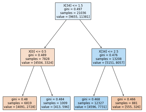 Note. A decision tree with a tree depth of two has fewer decision nodes and is more interpretable.
4.4.1.6. Random Forest Classifier Combining a baseline decision tree model with a bootstrapped aggregation (bagging) allowed for the first ensemble method of the random forest classifier to be introduced. The model was iterated through a list of maximum depths ranging from fifteen to twenty and trained and with the gini and entropy hyperparameters.
4.4.1.7. XGBoost. XGBoost was trained on the dataset for its scalability in a wide variety of end-to-end classification tasks. Parallelized computing allows for the algorithm to run “more than ten times faster than existing popular solutions on a single machine and scales to billions of examples in distributed or memory-limited settings” (Chen & Guestrin, 2016, p.1). Computational efficiency in conjunction with model complexity is an optimal solution. Therefore, this gradient boosting ensemble method was chosen to supplement the preceding tree-based classifiers. The model can be summarized in the following equation.
\[ \hat y_i = \large \sum_{k=1}^k f_k(x_i), f_k \epsilon \mathcal{F} \] where output \(\hat{y}_i\) is predicted, k is the number of trees, and \(f\) is the functional space of \(\mathcal{F}\).
4.4.1.8. Model deployment. The XGBoost model was used to predict the probability of violent crime occurring on Los Angeles streets. The model predictions were joined back to the Los Angeles streets GIS dataset and uploaded to a web application for final deployment. Figure 6 depicts the probability of violent crime by street.
Figure 6
Violent Crime Heat Map
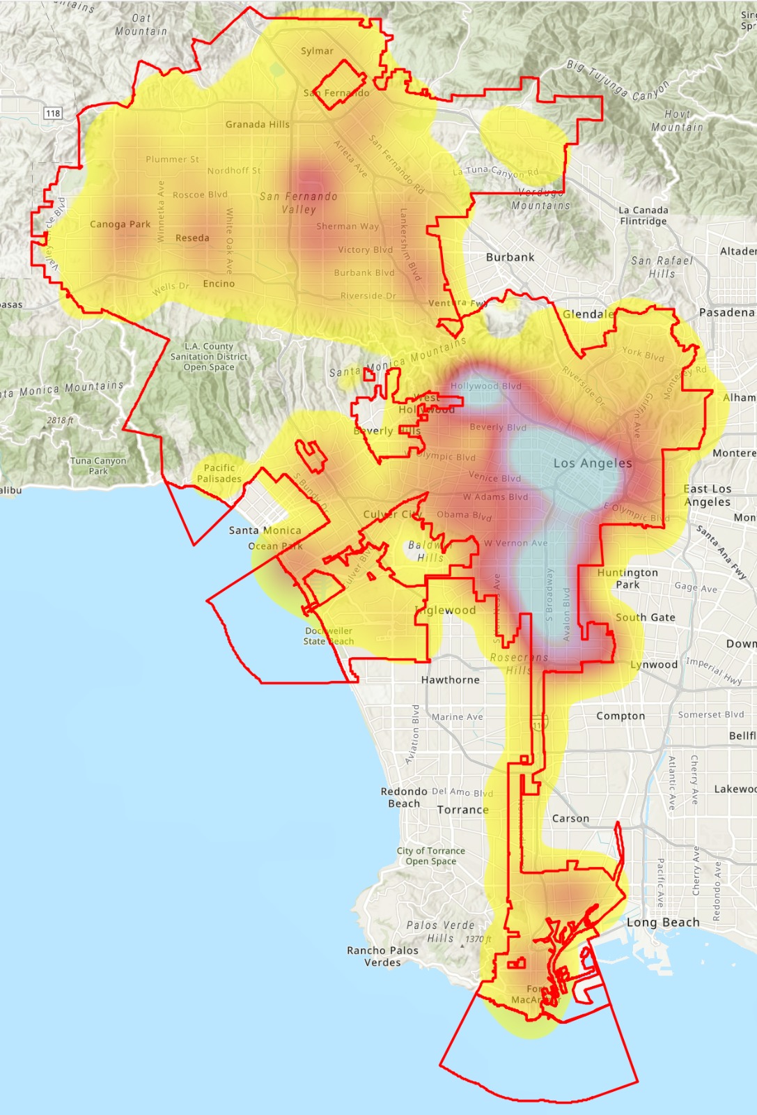
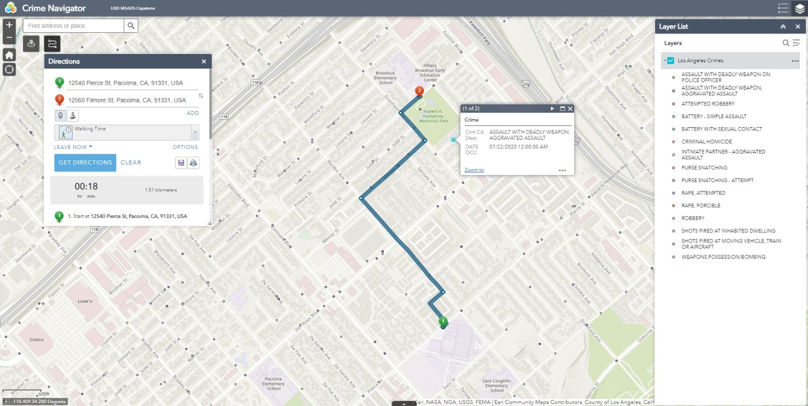
Both probability and crime frequency over the past six months were used to flag dangerous streets for routing purposes. The flagged streets act as barriers within the web mapping application routing function. When locations are selected within the application, the shortest route between those locations is created — avoiding the streets flagged as dangerous. Figure 7 shows the final deployment web application.
Figure 7
ArcGIS Web Application
5 Results and Findings
Figure 8 illustrates the actual versus predicted counts for the XGBoost model.
Figure 8
XGBoost Confusion Matrix

Note. The XGBoost model shows 5,121 true positives (contributing to the highest sensitivity of all models).
Next, ROC Curves were plotted for each respective model to assess model performance. Figure 9 illustrates the area captured under each curve.
Figure 9
Area Under Receiver Operating Characteristic

Note. The XGBoost model shows the highs AUC score of 0.94.
5.1 Evaluation of Results
One metric alone should not drive performance evaluation. Therefore, accuracy, precision, recall, f1, and AUC scores were considered.
Table 3 shows the performance metrics for all trained and validated models in order that they were implemented and AUC scores in comparison with each model’s mean squared errors.
Table 3
Performance Metrics
|
Model |
Accuracy |
Precision |
Recall |
F1-score |
AUC |
MSE |
|---|---|---|---|---|---|---|
|
QDA |
0.4953 |
0.6071 |
0.1748 |
0.2715 |
0.5361 |
0.4883 |
|
Decision Tree |
0.6217 |
0.6233 |
0.7499 |
0.6807 |
0.6413 |
0.2336 |
|
Logistic Regression |
0.6988 |
0.7013 |
0.7665 |
0.7324 |
0.7772 |
0.1925 |
|
Random Forest |
0.8496 |
0.8376 |
0.8936 |
0.8647 |
0.9185 |
0.1327 |
|
XGBoost |
0.8833 |
0.8845 |
0.9007 |
0.8925 |
0.9357 |
0.0918 |
XGBoost outperformed all other models based on highest accuracy (0.8885), precision (0.8894), recall (0.9053), and f1-score (0.8972). Moreover, it showed the highest AUC score (0.8871) and lowest mean squared error (0.1115).
6 Discussion
The results for the initial testing of both the model and the GIS routing application have been positive. The model performed well in predicting the test data and once the data were joined back to the original geographic features, the predictions were in-line with expectations for the area. Similar projects concluded that other factors, such as time and distance, should also be incorporated into determining the safest route because the amount of time spent in a high crime area could be a factor in overall safety. Taking this into account, time, distance, and mode of transportation were also incorporated into the final GIS application as choices for the end user. The number of historical incidents was also an important factor to consider when determining which streets to avoid, because it helps provide more granularity in situations where streets have similar predictive outcomes. Incident data classified by time of day was added to the GIS application to enhance clarity and situational awareness. Predicting crime is a difficult endeavor because the factors that dictate where and why crime occurs are constantly changing. Model predictions can help provide insights into where crime may occur; however, by incorporating other pertinent information a more meaningful picture may emerge regarding the reality of safety in any given area.
6.1 Conclusion
During this project, some key considerations came to light regarding safely navigating potentially dangerous areas. Model outcomes alone would likely not be sufficient for ensuring safety with a significant degree of confidence. While historical crime data adds a layer of information, more information may be required to get a complete picture of safety in a particular area. There may be other factors associated with location and crime that contribute to safety. For example, lighting and the presence of other people are not currently considered but could be useful for evaluating safety. To avoid a potentially dangerous main street, an individual may decide to alter their course and travel along an adjacent side street. An argument could be made that the side street may be more dangerous than the main street because of unknown factors. The side street could also have less crime because it is traveled less often. It can be difficult to identify the main factors that contribute to safety because those factors may be different depending on location. Ultimately, there may not be a safe route, and the safest option is to avoid the area altogether. Routing applications, like the one created for this project, are best suited for planning purposes so that individuals can identify safer pedestrian routes prior to traveling.
6.2 Recommended Next Steps/Future Studies
Ancillary data can provide additional insight in determining safer routes in the absence of historical crime data. It is equally important to consider that too much data can make interpretation and decision making more difficult. Extensive testing and further research may be necessary to determine the most important considerations for pedestrian safety to ensure only the most useful data are included.
References
Bura, D., Singh, M., & Nandal, P. (2019). Predicting Secure and Safe Route for Women using Google Maps. 2019 International Conference on Machine Learning, Big Data, Cloud and Parallel Computing (COMITCon).-
https://doi.org/10.1109/comitcon.2019
-
https://doi.org/10.1145/2939672.2939785
City of Los Angeles. (2022). Street Centerline [Data set]. Los Angeles Open Data. https://data.lacity.org/City-Infrastructure-Service-Requests/Street-Centerline/7j4e-nn4z
City of Los Angeles. (2022). City Boundaries for Los Angeles County [Data set]. Los Angeles Open Data. https://controllerdata.lacity.org/dataset/City-Boundaries-for-Los-Angeles-County/sttr-9nxz
Kuhn, M., & Johnson, K. (2016). Applied Predictive Modeling. Springer. https://doi.org/10.1007/978-1-4614-6849-3
Levy, S., Xiong, W., Belding, E., & Wang, W. Y. (2020). SafeRoute: Learning to Navigate Streets Safely in an Urban Environment. ACM Transactions on Intelligent Systems and Technology, 11(6), 1-17.-
https://doi.org/10.1145/3402818
Lopez, G., 2022, April 17. A Violent Crisis. The New York Times. https://www.nytimes.com/2022/04/17/briefing/violent-crime-ukraine-war-week-ahead.html.
Los Angeles Police Department. (2022). Crime Data from 2020 to Present [Data set]. https://data.lacity.org/Public-Safety/Crime-Data-from-2020-to-Present/2nrs-mtv8
Pavate, A., Chaudhari, A., & Bansode, R. (2019). Envision of Route Safety Direction Using Machine Learning. Acta Scientific Medical Sciences, 3(11), 140–145. https://doi.org/10.31080/asms.2019.03.0452
Pedregosa, F., Varoquaux, G., Gramfort, A., Michel, V., Thirion, B., Grisel, O., Blondel, M., Prettenhofer, P., Weiss R., Dubourg, V., Vanderplas, J., Passos, A., Cournapeau, D., Brucher, M., Perrot, M.,-
and Duchesnay, E. (2011). Scikit-learn: Machine learning in Python. Journal of Machine Learning Research, 12(Oct), 2825–2830.
-
http://ijcsit.com/docs/Volume%207/vol7issue3/ijcsit20160703106.pdf
Vandeviver, C. (2014). Applying Google Maps and Google Street View in criminological research. Crime Science, 3(1). https://doi.org/10.1186/s40163-014-0013-2
Wang, Y. Li, Y., Yong S., Rong, X., Zhang, S. (2017). Improvement of ID3 algorithm based on simplified information entropy and coordination degree. 2017 Chinese Automation Congress (CAC), 1526-1530.-
https://doi.org/10.1109/CAC.2017.8243009