Modeling
Team Members: Leonid Shpaner, Christopher Robinson, and Jose Luis Estrada
This notebook culminates with modeling, validation, and evaluation.
from google.colab import drive
drive.mount('/content/drive', force_remount=True)
%cd /content/drive/Shared drives/Capstone - Best Group/GitHub Repository/navigating_crime/Code Library
####################################
## import the requisite libraries ##
####################################
import os
import csv
import pandas as pd
import numpy as np

# import plotting libraries
import matplotlib.pyplot as plt
import seaborn as sns

# import miscellaneous libraries
from prettytable import PrettyTable  # for creating tables

# import modeling libraries
import scipy as sp # for extracting pearson correlation coefficient
from sklearn.linear_model import LogisticRegression
from sklearn.ensemble import RandomForestClassifier, ExtraTreesClassifier
from xgboost import XGBClassifier

from sklearn.discriminant_analysis import QuadraticDiscriminantAnalysis
from sklearn.tree import DecisionTreeClassifier

from sklearn import metrics, tree
from sklearn.metrics import roc_curve, auc, mean_squared_error,\
precision_score, recall_score, f1_score, accuracy_score,\
confusion_matrix, plot_confusion_matrix, classification_report

import warnings
# suppress warnings for cleaner output
warnings.filterwarnings('ignore')
# suppress future warnings for cleaner output
warnings.filterwarnings(action='ignore', category=FutureWarning)
# set random state for reproducibility
rstate = 222
# check current working directory
current_directory = os.getcwd()
current_directory
Assign Paths to Folders
# path to data folder
data_folder = '/content/drive/Shareddrives/Capstone - Best Group/' \
            + '/GitHub Repository/navigating_crime/Data Folder/'

# path to the training file
train_path = '/content/drive/Shareddrives/Capstone - Best Group/' \
           + '/GitHub Repository/navigating_crime/Data Folder/train_set.csv'

# path to the validation file
valid_path = '/content/drive/Shareddrives/Capstone - Best Group/' \
           + '/GitHub Repository/navigating_crime/Data Folder/valid_set.csv'

# path to the feature engineered original dataframe (for eda purposes)
data_frame = '/content/drive/Shareddrives/Capstone - Best Group/' \
           + 'Final_Data_20220719/df.csv'

# path to the validation file
test_path = '/content/drive/Shareddrives/Capstone - Best Group/' \
          + '/GitHub Repository/navigating_crime/Data Folder/test_set.csv'

# path to the image library
model_image_path = '/content/drive/Shareddrives/Capstone - Best Group/' \
                 + '/GitHub Repository/navigating_crime/Image Folder/' \
                 + 'Modeling Images'
# bring in original dataframe only for join purposes
train_set = pd.read_csv(train_path).set_index('OBJECTID')
valid_set = pd.read_csv(valid_path).set_index('OBJECTID')
test_set = pd.read_csv(test_path).set_index('OBJECTID')
# print the training
print('The training set is', train_set.shape[0], 'rows and', train_set.shape[1],
      'columns.')
print('The validation set is', valid_set.shape[0], 'rows and', valid_set.shape[1],
      'columns.')
print('The testn set is', test_set.shape[0], 'rows and', test_set.shape[1],
      'columns.')
# subset the inputs for train and val (X_train, y_train, respectively) as
# only input features, omitting the crime code truthing columns.
X_train = train_set.drop(columns=['Crime_Code'])
y_train = pd.DataFrame(train_set['Crime_Code'])

X_val = valid_set.drop(columns=['Crime_Code'])
y_val = pd.DataFrame(valid_set['Crime_Code'])
Models
Quadratic Discriminant Analysis (QDA)
A form of nonlinear discriminant analysis (Quadratic Discriminant Analysis) is used with an assumption that the data follows a Gaussian distribution such that a "class-specific covariance structure can be accommodated" (Kuhn & Johnson, 2016, p. 330). This method is used to improve performance over a standard Linear Discriminant Analysis (LDA) whereby the class boundaries are linearly separable. It does not require hyperparameters because it has a closed-form solution (Pedregosa et al., 2011).
qda = QuadraticDiscriminantAnalysis()
qda.fit(X_train, y_train)

# Predict on val set
qda_pred = qda.predict(X_val)
# extract predicted probabilities for validation set
qda_proba = qda.predict_proba(X_val)[:,1]
Logistic Regression
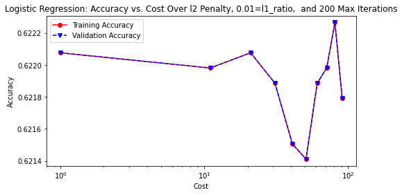
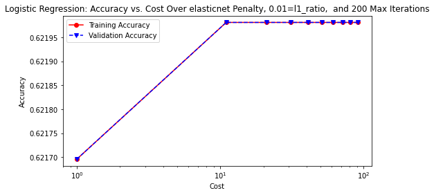
Logistic regression is deployed next for its ability to handle binary classification tasks with relative ease. The generalized linear model takes the following form:
$$y = \beta_0 + \beta_1x_1 +\beta_2x_2 +\cdots+\beta_px_p + \varepsilon$$Describing the relationship between several important coefficients and features in the dataset can be modeled parametrically in the following form:
$$(\hat{\text{Crime Code}}) = \frac{\text{exp}(b_0+{b_1(\text{Victim Age}})+{b_2(\text{Month}})+b_3(\text{Victim Sex})+\cdot\cdot\cdot+b_px_p)}{1+\text{exp}(b_0+{b_1(\text{Victim Age}})+{b_2(\text{Month}})+b_3(\text{Victim Sex})+\cdot\cdot\cdot+b_px_p)}$$The model is iterated through a list of cost penalties from 1 to one-hundred and trained with the following hyperparameters. Solvers used were lbfgs and saga. The l1-ratio and maximum iterations (max_iter) remained constant at a rate of 0.01, and 200, respectively.
# logistic regression function with hyperparameter tuning
def lr_hp(solver, penalty, l1_ratio, max_iter, rstate):
    '''
    Inputs:
        solver = hyperparameter (default is 'lbfgs')
        penalty = norm (i.e., l1, l2, etc.,)
        ratio = l1_ratio
        cost = C, a positive float (inverse of regularization)
        maxiter = number of maximum iterations
        rstate = random state for reproducibility
    '''
    # manually tuning the logistic regression model
    C = list(range(1, 100, 10))  #cost various in a range from 1-100 by 10
    LRtrainAcc = []
    LRvalAcc = []
    for cost in C:
        lr = LogisticRegression(solver=solver, penalty=penalty, l1_ratio=l1_ratio,
                                C=cost, max_iter=max_iter, random_state=rstate)
        lr.fit(X_train, y_train) # fit the model

        lr_pred_train = lr.predict(X_train)  # Predict on train set
        tuned_lr = lr.predict(X_val)         # Predict on val set
        # append accuracy score to train and val, respectively and show over
        # each respective cost
        LRtrainAcc.append(accuracy_score(y_val, tuned_lr))
        LRvalAcc.append(accuracy_score(y_val, tuned_lr))
        print('Cost = %2.2f \t Validation Accuracy = %2.2f \t Training ' \
              'Accuracy = %2.2f'% (cost,accuracy_score(y_val, tuned_lr),
                               accuracy_score(y_train, lr_pred_train)))

    # plot training and validation accuracy by cost
    fig, ax = plt.subplots(figsize=(8, 4))
    ax.plot(C, LRtrainAcc, 'ro-', C, LRvalAcc,'bv--')
    ax.legend(['Training Accuracy','Validation Accuracy'])
    ax.set_title(f'Logistic Regression: Accuracy vs. Cost Over {penalty}' \
    + f' Penalty, {l1_ratio}=l1_ratio,  and {max_iter} Max Iterations')
    # plt.title('Logistic Regression: Accuracy vs. Cost')
    ax.set_xlabel('Cost'); ax.set_xscale('log')
    ax.set_ylabel('Accuracy')

    # accuracy and classification report (tuned model)
    print()
    print('Tuned Logistic Regression Model')
    print('Accuracy Score')
    print(accuracy_score(y_val, tuned_lr))
    print('Classification Report \n', classification_report(y_val, tuned_lr))
# tune the Logistic Regression with 'lbfgs' solver, 'l2' penalty,
# 'l1_ratio' of 0.01, and 200 'max_iter'
lr_hp(solver='lbfgs', penalty='l2', l1_ratio=0.01, max_iter=200, rstate=rstate)
# save the accuracy plot onto image path
plt.savefig(model_image_path + '/log_reg1_accuracy.png', bbox_inches='tight')
# tune the Logistic Regression with 'saga' solver, 'elasticnet' penalty,
# 'l1_ratio' of 0.01, and 200 'max_iter'
lr_hp(solver='saga', penalty='elasticnet', l1_ratio=0.01, max_iter=200,
      rstate=rstate)
# save the accuracy plot onto image path
plt.savefig(model_image_path + '/log_reg2_accuracy.png', bbox_inches='tight')
# train and predict final LogisticRegression model
lr = LogisticRegression(solver='saga', penalty='elasticnet', l1_ratio=0.01,
                        max_iter=200, random_state=rstate)
# fit the logistic regression model
lr.fit(X_train, y_train)
# Predict on val set
lr_pred = lr.predict(X_val)
# extract predicted probabilities for validation set
lr_proba = lr.predict_proba(X_val)[:, 1]
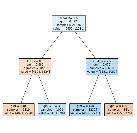
Decision Tree Classifier
The remainder of the modeling stage commences with the application of tree-based classifiers. Basic classification trees facilitate data partitioning "into smaller, more homogeneous groups" (Kuhn & Johnson, 2016, p. 370). Instantiating a Decision Tree Classifier at a maximum depth (max_depth) of 2 is a good baseline for illustrating the effects of a minimum sample split to arrive at a pure node, but a more realistic depth of fifteen provides a more realistic and interpretable framework from which to assess subsequent classifiers with. No other hyperparameters are tuned.
# assign new variable to decision tree classifier and set max_depth=2
# for small tree depth size such that the tree can be effectively plotted
dec_tree = DecisionTreeClassifier(max_depth=2)
# fit the tree
dec_tree.fit(X_train, y_train)
# Predict on val set
dec_tree_pred =  dec_tree.predict(X_val)
# extract predicted probabilities for validation set
dec_tree_proba = dec_tree.predict_proba(X_val)[:,1]
# plot the decision tree at a max_depth=2
fig, ax = plt.subplots(figsize = (10,10))

short_tree = tree.plot_tree(dec_tree, filled=True)
# save the accuracy plot onto image path
plt.savefig(model_image_path + '/decision_tree.png', bbox_inches='tight')
# assign new variable to decision tree classifier and set max_depth=15
tree = DecisionTreeClassifier(max_depth=15)
# fit the decision tree
tree.fit(X_train, y_train)
# Predict on val set
tree_pred =  tree.predict(X_val)
# extract predicted probabilities for validation set
tree_proba = tree.predict_proba(X_val)[:,1]
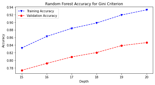
Random Forest Classifier
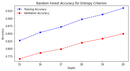
Combining a baseline decision tree model with a bootstrapped aggregation (bagging) allowed for the first ensemble method of the Random Forest Classifier to be introduced. The model was iterated through a list of maximum depths ranging from fifteen to twenty and trained and with the gini and entropy hyperparameters.
# random forest function with hyperparameter tuning
def rf_hp(criterion, rstate):
    '''
    Inputs:
        criterion: used to measure split quality; gini is default
        rstate: random state
    '''
    # Random Forest Tuning (Manual)
    rf_train_accuracy = []
    rf_val_accuracy = []
    # max_depth various from 15-20 in a for loop
    max_depth = list(range(15, 21))
    for n in max_depth:
        rf = RandomForestClassifier(max_depth=n, criterion=criterion,
                                    random_state=rstate)
        rf = rf.fit(X_train, y_train) # fit the classifier
        rf_pred_train = rf.predict(X_train) # predict on training set
        rf_pred_val = rf.predict(X_val) # predict on validation set
        # append accuracy score to train and val, respectively and show over
        # each respective max_depth
        rf_train_accuracy.append(accuracy_score(y_train, rf_pred_train))
        rf_val_accuracy.append(accuracy_score(y_val, rf_pred_val))
        print('Max Depth = %2.0f \t val Accuracy = %2.2f \t' \
              'Training Accuracy = %2.2f'% (n, accuracy_score(y_val,
                                                              rf_pred_val),
                                            accuracy_score(y_train,
                                                           rf_pred_train)))
    # plot training and validation accuracy
    fig, ax = plt.subplots(figsize=(8, 4))
    ax.plot(max_depth, rf_train_accuracy, 'bv--', label='Training Accuracy')
    ax.plot(max_depth, rf_val_accuracy, 'ro--', label='Validaiton Accuracy')
    ax.legend(['Training Accuracy','Validation Accuracy'])
    ax.set_title(f'Random Forest Accuracy for {criterion.capitalize()}' + \
                 ' Criterion')
    ax.set_xlabel('Depth')
    ax.set_ylabel('Accuracy')

    # accuracy and classification report
    print()
    print('Tuned Random Forest Model')
    print('Accuracy Score', '\n')
    print(accuracy_score(y_val, rf_pred_val))
    print('Classification Report \n',
          classification_report(y_val, rf_pred_val))
# run the random forest function, varying over max_depth of 15-20 as defined
# in rf_hp function
rf_hp('gini', rstate)
# save the accuracy plot onto image path
plt.savefig(model_image_path + '/rand_forest_gini_accuracy.png',
            bbox_inches='tight')
# run the random forest function with entropy criterion, varying over max_depth
# of 15-20 as defined in rf_hp function
rf_hp('entropy', rstate)
# save the accuracy plot onto image path
plt.savefig(model_image_path + '/rand_forest_entropy_accuracy.png',
            bbox_inches='tight')
# train and predict final RandomForest model
rf = RandomForestClassifier(max_depth=20, criterion='entropy',
                            random_state=rstate)
rf.fit(X_train, y_train) # fit the classifier
rf_pred = rf.predict(X_val) # Predict on val set
# extract predicted probabilities for validation set
rf_proba = rf.predict_proba(X_val)[:, 1]
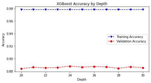
XGBoost
XGBoost is the final model trained on the dataset for its scalability in a wide variety of end-to-end classification tasks. Parallelized computing allows for the algorithm to run "more than ten times faster than existing popular solutions on a single machine and scales to billions of examples in distributed or memory-limited settings" (Chen & Guestrin, 2016). Therefore, this gradient boosting ensemble method was chosen to supplement the preceding tree-based classifiers.
The model can be summarized in the following equation:
$$\hat y_i = \large \sum_{k=1}^k f_k(x_i), f_k \epsilon \mathcal{F} $$where output $\hat y_i$ is predicted via a summation of $k$ number of trees, where $f$ is the functional space of $\mathcal{F}$.
def xgb_hp(lr, rstate):
    '''
    Inputs:
        lr: learning rate
        rstate: random state for reproducibility
    '''
    # XGBoost tuning
    xgb_train_accuracy = []
    xgb_val_accuracy = []
    max_depth = list(range(20, 31)) # max depth from 20-30
    for n in max_depth:
        xgb = XGBClassifier(max_depth=n, tree_method='hist', # speeds up time
                            learning_rate=lr, n_estimators=250,
                            random_state=rstate, n_jobs=-1) # uses all cores
        xgb = xgb.fit(X_train, y_train) # fit the xgboost classifier
        xgb_pred_train = xgb.predict(X_train) # predict on training set
        xgb_pred_val = xgb.predict(X_val)     # predict on validation set
        # append accuracy score to train and val, respectively and show over
        # each respective max_depth
        xgb_train_accuracy.append(accuracy_score(y_train, xgb_pred_train))
        xgb_val_accuracy.append(accuracy_score(y_val, xgb_pred_val))
        print('Max Depth = %2.0f \t Validation Accuracy = %2.2f \t' \
              'Training Accuracy = %2.2f' %(n, accuracy_score(y_val,
                                            xgb_pred_val),
                                            accuracy_score(y_train,
                                                           xgb_pred_train)))
    # plot training and validation accuracy
    fig, ax = plt.subplots(figsize=(8, 4))
    ax.plot(max_depth, xgb_train_accuracy, 'bv--', label='Training Accuracy')
    ax.plot(max_depth, xgb_val_accuracy, 'ro--', label='Validation Accuracy')
    ax.set_title('XGBoost Accuracy by Depth')
    ax.set_xlabel('Depth')
    ax.set_ylabel('Accuracy')
    plt.legend()

    # accuracy and classification report
    print()
    print('Tuned XGBoost Model')
    print('Accuracy Score', '\n')
    print(accuracy_score(y_val, xgb_pred_val))
    print('Classification Report \n', classification_report(y_val, xgb_pred_val))
# run the xgboost function with 0.5 learning rate, varying over max_depth
# of 20-30 as defined in xgb_hp function
xgb_hp(lr=0.5, rstate=rstate)
# save the accuracy plot onto image path
plt.savefig(model_image_path + '/xgboost_accuracy.png', bbox_inches='tight')
# train and predict final XGBoost model
xgb = XGBClassifier(max_depth=31, lr=0.5, random_state=rstate)
xgb.fit(X_train, y_train) # fit the classifier
xgb_pred = xgb.predict(X_val) # Predict on val set
# extract predicted probabilities for validation set
xgb_proba = xgb.predict_proba(X_val)[:, 1]
Model Evaluation
Confusion Matrices
fig, axes = plt.subplots(nrows=2, ncols=2, figsize=(12, 12))
flat = axes.flatten()
fig.tight_layout(w_pad=2, h_pad= 6)

# Quadratic Discriminant Analysis confusion matrix is omitted since its results
# are at the baseline level
# Logistic Regression confusion matrix
plot_confusion_matrix(lr, X_val, y_val, ax=flat[0])
flat[0].set_title('Logistic Regression')

# Decision Tree confusion matrix
plot_confusion_matrix(tree, X_val, y_val, ax=flat[1])
flat[1].set_title('Decision Trees')

# Random Forest confusion matrix
plot_confusion_matrix(rf, X_val, y_val, ax=flat[2])
flat[2].set_title('Random Forest Classifier')

# XGBoost confusion matrix
plot_confusion_matrix(xgb, X_val, y_val, ax=flat[3])
flat[3].set_title('XGBoost')

# save the confusion matrices onto image path
plt.savefig(model_image_path + '/confusion_matrices.png', bbox_inches='tight')

plt.show()
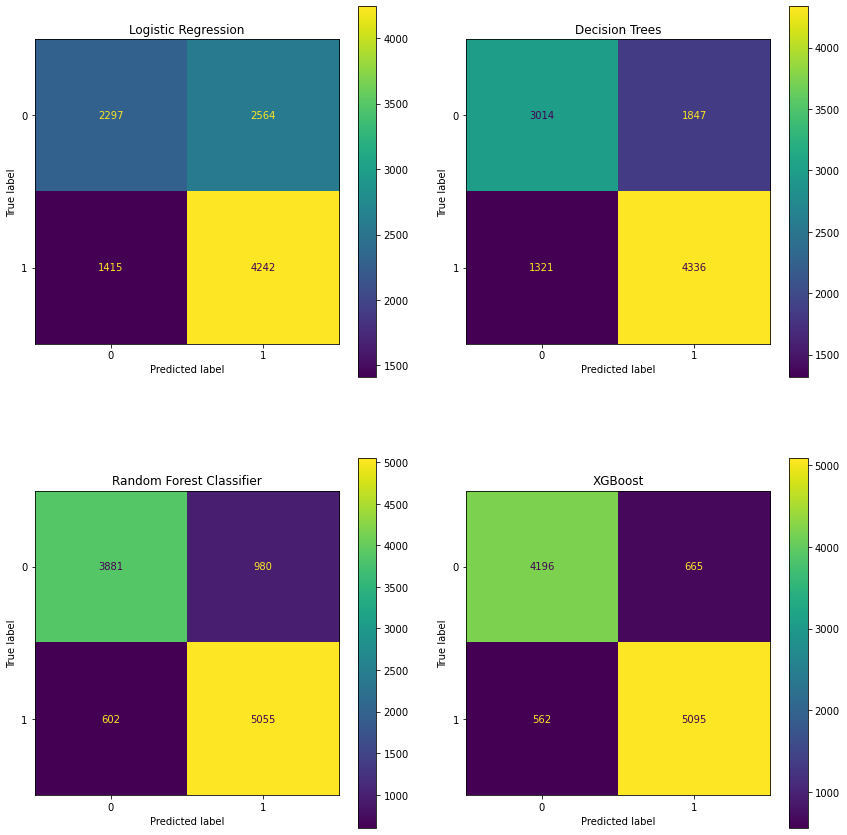
The XGBoost model shows 5,121 true positives (contributing to the highest sensitivity of all models).
ROC Curves
ROC Curves were plotted for each respective model to assess model performance.
# function for plotting roc curves
def roc_plots(est_name, name, ax=None):
    '''
    Inputs:
        est_name: model name (variable)
        name: model name (string)
        ax=None: axis
    Output:
        ax: axis
    '''
    roc = metrics.roc_curve(y_val, est_name)
    fpr,tpr,thresholds = metrics.roc_curve(y_val, est_name)
    auc = metrics.auc(fpr, tpr)

    if ax is None:
        fig, ax = plt.subplots(figsize=(15, 10))
        plt.title('')
        plt.xlabel('')
        plt.ylabel('')
        plt.legend('')
    ax.plot(fpr, tpr, label=f'{name}; AUC = {auc:.2}', linewidth=3)
    ax.plot([0, 1], [0, 1], linestyle='--', color='#174ab0')
    return ax
# create a dataframe for the models that were run
models = pd.DataFrame({'qda': qda_proba, 'log': lr_proba, 'rf': rf_proba,
                       'tree': tree_proba, 'xgb': xgb_proba,
                       'y_val': y_val['Crime_Code'].values})

# save out the models into a .csv file to be used with dash plotly
models.to_csv(data_folder + 'models.csv', index=False)
# plot the roc curves using the roc_plots function
ax = roc_plots(est_name=qda_proba, name='QDA')
roc_plots(est_name=lr_proba, name='Logistic Regression', ax=ax)
roc_plots(est_name=tree_proba, name='Decision Trees', ax=ax)
roc_plots(est_name=rf_proba, name='Random Forest', ax=ax)
roc_plots(est_name=xgb_proba, name='XGBoost', ax=ax)
plt.title('ROC Curves', fontsize=18)
plt.xlabel('False Positive Rate', fontsize=18)
plt.ylabel('True Positive Rate', fontsize=18)
plt.legend(loc='lower right', fontsize=18);
# save the roc plot onto image path
plt.savefig(model_image_path + '/roc_curves.png', bbox_inches='tight')
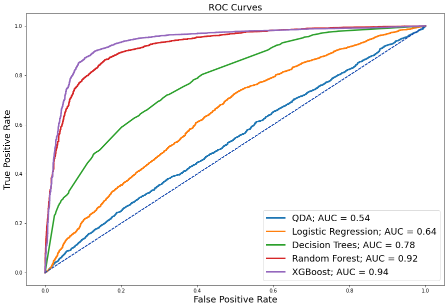
Determining the model for deployment involves a comprehensive inspection of all area under the receiver operating characteristic (AUROC) curves. As you can see here, we have our introductory QDA model with an auc of 0.54, which is barely above the baseline. Logistic regression makes a 10% improvement to an AUC of 0.64, followed by the Decision Tree that adds another 14% to an AUC of 0.78, and performance keeps improving, especially with these more complex tree-based classifiers, where we now see the best performing model of XGB with an auc of 0.94. However, sensitivity and false alarm rates should also be considered as additional measures of performance assessment.
Performance Metrics
# function that generates auc values for any given value
def roc_auc(est_name):
    '''
    Input:
        est_name: name of model(estimator/algorithn)
    Output:
        auc: auc score
    '''
    roc = metrics.roc_curve(y_val, est_name)
    fpr,tpr,thresholds = metrics.roc_curve(y_val, est_name)
    auc = metrics.auc(fpr, tpr)
    return auc
models = {'QDA': qda_proba, 'Logistic Regression': lr_proba,
          'Decision Tree': tree_proba, 'Random Forest': rf_proba,
          'XGBoost': xgb_proba}
metrics_dict = {}
for key, val in models.items():
    report = classification_report(y_val, 1*(val > 0.5), output_dict=True)
    metrics_dict[key] = [round(report['accuracy'],4),
                         round(report['1']['precision'],4),
                         round(report['1']['recall'],4),
                         round(report['1']['f1-score'],4) ]
table1 = PrettyTable()
table1.field_names = ['Model', 'Validation Accuracy', 'Precision',
                      'Recall', 'F1-score']

for key, val in metrics_dict.items():
    table1.add_row([key] + val)
print(table1)

# Mean-Squared Errors
table2 = PrettyTable()
table2.field_names = ['Model', 'AUC', 'MSE']

for key, val in models.items():
    table2.add_row([key,  round(roc_auc(val),4), round(mean_squared_error(y_val, val),4)])
print(table2)
One metric alone should not drive performance evaluation. Therefore, accuracy, precision, recall, f1, and AUC scores were considered. These tables show the performance metrics for all trained and validated models in order that they were implemented and AUC scores in comparison with each model’s mean squared errors. XGBoost outperformed all other models based on highest accuracy (0.8885), precision (0.8894), recall (0.9053), and f1-score (0.8972). Moreover, it showed the highest AUC score (0.8871) and lowest mean squared error (0.1115).
XGBoost Predictions
The predictions from the XGBoost model are joined back to the validation holdout set on the index (OBJECTID) such that these predictions can be further used to assess model performance on categorical variables of interest.
# create copy of validation set to join xgb model predictions to
df_predictions_xgb = valid_set.copy()
# join the xgb model predictions to validation set copy
df_preds_xgb = pd.concat([X_val, y_val], axis=1)
df_preds_xgb['Predictions'] = xgb_proba
df_preds_xgb.head() # inspect xgboost predictions
# write out the xgboost predictions to file on path
df_preds_xgb.to_csv(data_folder + 'df_preds_xgb.csv')
# function for plotting categorical column roc curves
def plot_roc_preds(df, title, column):
    '''
    This function creates roc curves plot for predictions
    Inputs:
        df_preds: dataframe with appended predictions
        title: title of the plot
        column: column to look at (i.e., 'Age', etc.)
        dictionary: key-value pair mapping for column
    '''

    # filter by each unique value in column
    for value, filtered_preds in df.groupby(column):
        filtered_preds = df[df[column]==value]

        if filtered_preds.shape[0] > 0:
            # plot roc curve
            fpr, tpr, thresholds = metrics.roc_curve(filtered_preds['Crime_Code'],
                                                     filtered_preds['Predictions'])
            y_preds = df[df[column]==value]['Predictions'] # predictions column
            y_true = df[df[column]==value]['Crime_Code'] # ground truth column
            count = len(y_true)
            len_h0 = len(y_true[y_true==0]) # where ground truth = 0
            len_h1 = len(y_true[y_true==1]) # where ground truth = 1

            if len_h0 and len_h1:
                roc_auc = metrics.auc(fpr, tpr)
                # make the plot
                plt.rcParams["figure.figsize"] = [16, 10] # plotting figure size
                plt.title(title)
                plt.plot(fpr, tpr, label = f'AUC for {value} = {roc_auc:.3f},'
                                          f' count: {len(y_true)}, H0: {len_h0},'
                                          f' H1: {len_h1}')
                plt.plot([0, 1], [0, 1], 'r--')
                plt.xlim([0, 1])
                plt.ylim([0, 1])
                plt.xlabel('False Positive Rate')
                plt.ylabel('True Positive Rate')
                plt.legend(loc="lower right")
# save entire original dataframe (pre-modeling) to new variable for subsequent
# joining/concatenation based on 'OBJECTID' index
df = pd.read_csv(data_frame).set_index('OBJECTID')
# join columns of interest from eda datframe to the prediction dataframe
# for further ROC Curve analysis
df_preds_roc= df_preds_xgb.join(df[['Type', 'age_bin', 'Victim_Sex',
                                    'Victim_Desc', 'Time_of_Day', 'Month',
                                    'AREA_NAME']], how='left')
# drop individual streets from new dataframe, since we are not interested in
# investing performance operating points at this granularity. However,
# street tpes, age groups, time of day, and month are retained such that
# this analysis can be made
df_preds_roc = df_preds_roc.drop(columns=['77th_Street', 'Central', 'Devonshire',
                                          'Foothill', 'Harbor', 'Hollenbeck',
                                          'Hollywood', 'Mission', 'N_Hollywood',
                                          'Newton','Northeast', 'Olympic',
                                          'Pacific', 'Rampart', 'Southeast',
                                          'Southwest','Topanga', 'Van_Nuys',
                                          'West_LA', 'West_Valley', 'Wilshire',
                                          # remove individual time of day cols
                                          # since these are already contained
                                          # within 'Time_of_Day' col
                                          'Afternoon', 'Evening', 'Morning',
                                          'Night',
                                          # remove individual street type cols
                                          # since these are already contained
                                          # within 'Type' column
                                          'Alley', 'Driveway', 'Park_Playground',
                                          'Parking_Lot', 'Sidewalk', 'Street',
                                          'Vacant_Lot',
                                          # remove 'Month_No' col since relvant
                                          # info is contained within 'Month' col
                                          'Month_No',
                                          # remove 'Vict_Age' since we have
                                          # binned it as 'age_bin'
                                          'Vict_Age',
                                          # drop gender in lieu of 'Victim_Sex'
                                          'Gender'],
                                          errors='ignore')

# create dictionary for renaming certain columns
options = {'age_bin': 'Age Bin',  'Type': 'Type', 'Victim_Sex': 'Victim Sex',
           'Victim_Desc': 'Victim Descent', 'Time_of_Day': 'Time of Day',
           'Month': 'Month', 'AREA_NAME': 'Area Name', 'Premises': 'Premises'}

df_preds_roc = df_preds_roc.rename(columns=options) # rename the columns
# write out the df_preds (+) joined columns of interest file to csv on path
df_preds_roc.to_csv(data_folder + 'df_preds_roc.csv', index=False)
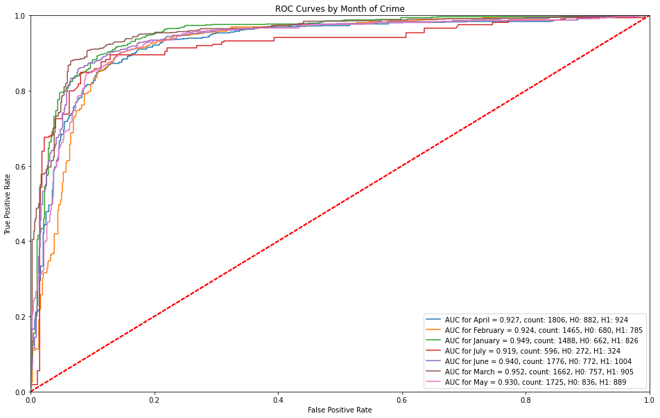
ROC Curves by Month of Crime
Month over month, the operating points of the ROC are consistent. However, it is interesting to note that the month of March captures a high sensitivity for predicting serious crimes (~50%) before receiving any false alarms.
# roc curves by month of crime
plot_roc_preds(df_preds_roc, 'ROC Curves by Month of Crime', 'Month')
# save the roc plot onto image path
plt.savefig(model_image_path + '/roc_by_month.png', bbox_inches='tight')
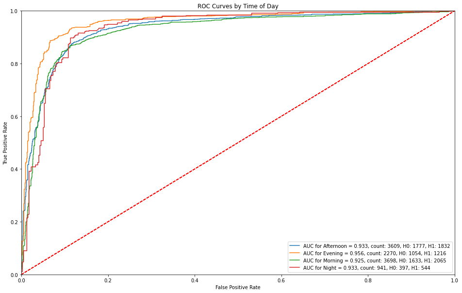
ROC Curves by Time of Day
Evening captures a higher sensitivity (true positive rate) prior to receiving any false alarms. Night predictions receive false alarms at a sensitivity of approximately 40%.
# roc curves by time of day
plot_roc_preds(df_preds_roc, 'ROC Curves by Time of Day', 'Time of Day')
# save the roc plot onto image path
plt.savefig(model_image_path + '/roc_by_time_of_day.png', bbox_inches='tight')
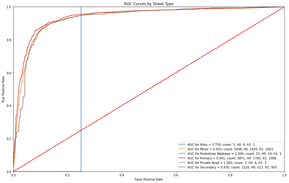
ROC Curves by Street Type
Alleys have an immediate false alarm of over 20% and no true positive rate. Otherways primary streets receive a higher sensitivity before countering with a false alarm rate (1-specificity).
# plot roc curves by street type
plot_roc_preds(df_preds_roc, 'ROC Curves by Street Type', 'Type')
# save the roc plot onto image path
plt.savefig(model_image_path + '/roc_by_street_type.png', bbox_inches='tight')
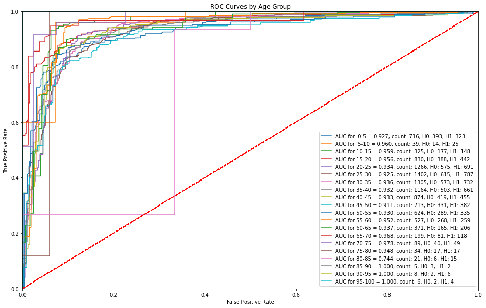
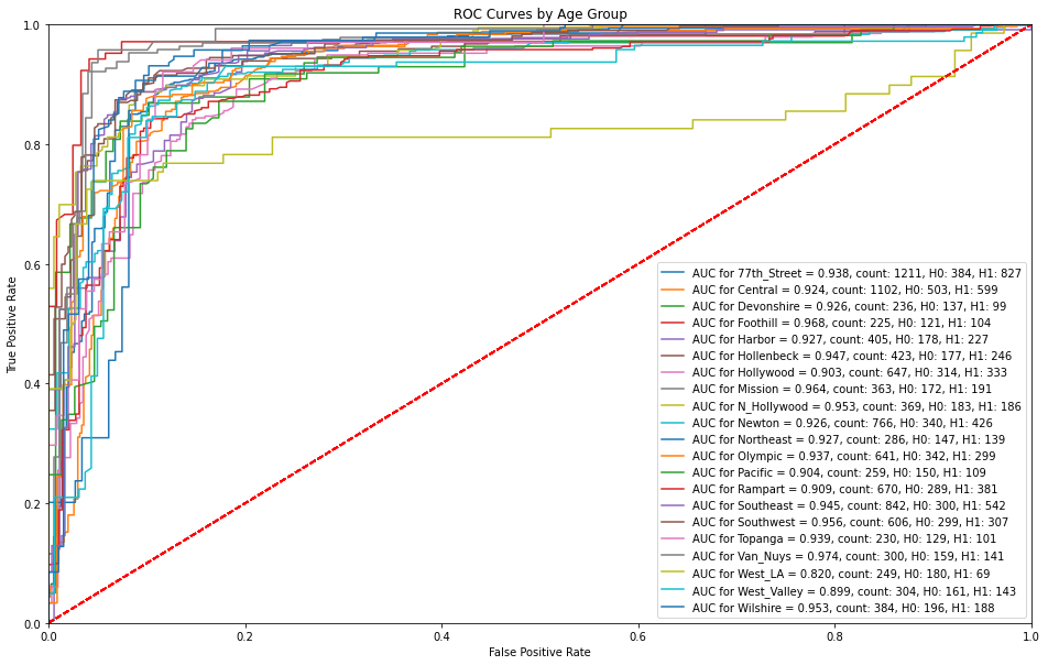
ROC Curves by Age Group
The XGBoost model is able to successfully make predictions with a high sensitivity without any false alarms with the exception of age bins of 75-80 and 85-90 where there are higher false alarms at lower sensitivities
# plot roc curves by street age group
plot_roc_preds(df_preds_roc, 'ROC Curves by Age Group', 'Age Bin')
# save the roc plot onto image path
plt.savefig(model_image_path + '/roc_by_age.png', bbox_inches='tight')
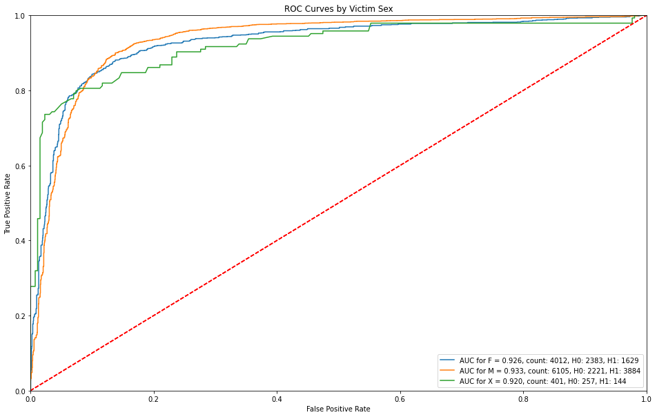
ROC Curves by Victim Sex
Victim sex is for the most part, consistent throughout, but those sexes that remain unknown have higher detection rates before getting any false alarms.
# plot roc curves by street sex
plot_roc_preds(df_preds_roc, 'ROC Curves by Victim Sex', 'Victim Sex')
# save the roc plot onto image path
plt.savefig(model_image_path + '/roc_by_sex.png', bbox_inches='tight')
ROC Curves by Area Name
In terms of location or specific areas in Los Angeles, North Hollywood stands out in terms of receiving higher false alarms with respect to lower sensitivities.
# plot roc curves by area name
plot_roc_preds(df_preds_roc, 'ROC Curves by Age Group', 'Area Name')
# save the roc plot onto image path
plt.savefig(model_image_path + '/roc_by_area.png', bbox_inches='tight')
Compare Predictions of Top Two Models
XGBoost was the top performing model in terms of AUC, accuracy, precision, recall, f1-score, and lowest mean-squared error. For comparison purposes, predictions are generated for the second best model (Random Forest).
# create new dataframe for random forest predictions as validation set copy to
# join model predictions on
df_predictions_rf = valid_set.copy()
df_preds_rf = pd.concat([X_val, y_val], axis=1) # join the model preds to df
df_preds_rf['Predictions'] = rf_proba
# save random forest predictions to .csv file on path
df_preds_rf.to_csv(data_folder + 'df_preds_rf.csv')
# create a new column of predictions for RF (for naming purposes)
df_preds_rf['Predictions_RF'] = df_preds_rf['Predictions']
# drop any other columns in the dataframe since only predictions are of interest
df_preds_rf_preds = df_preds_rf[['Predictions_RF', 'Crime_Code']]

# create a new column of predictions for XGB (for naming purposes)
df_preds_xgb['Predictions_XGB'] = df_preds_xgb['Predictions']
# drop any other columns in the dataframe since only predictions are of interest
df_preds_xgb_preds = df_preds_xgb[['Predictions_XGB']]
# join the prediction columns of XGB and RF dataframes, respectively
pred_comparison = df_preds_xgb_preds.join(df_preds_rf_preds, how='left')
pred_comparison.head()
# draw scatter plot comparing random forest predictions with xgboost,
# colored by ground truth (crime code) column
sns.scatterplot(data=pred_comparison, x=pred_comparison['Predictions_XGB'],
                y = pred_comparison['Predictions_RF'], hue='Crime_Code')

plt.title('RF and XGBoost Prediction Comparisons')
plt.xlabel('XGBoost Predictions')
plt.ylabel('Random Forest Predictions')

# call the scipy function for pearson correlation
r, p = sp.stats.pearsonr(x=pred_comparison['Predictions_XGB'],
                y = pred_comparison['Predictions_RF'])
# annotate the pearson correlation coefficient text to 2 decimal places
plt.text(.05, .8, 'r={:.2f}'.format(r),
            transform=ax.transAxes)

# save the prediction comparisons onto image path
plt.savefig(model_image_path + '/pred_comparisons_colored.png',
            bbox_inches = 'tight')
plt.show()
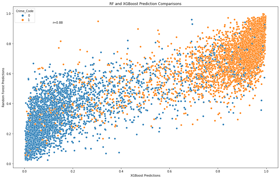
Note. Both models predictions are comparable at a Pearson correlation coefficient of r=0.84. Blue represents less serious crimes and orange represents more serious crimes.
XGBoost: Deployment - Training and Predicting on The Test Set
# read in the test set from path
test_set = pd.read_csv(test_path).set_index('OBJECTID')
# subset the inputs for test set (X_test, y_test, respectively) as
# only input features, omitting the crime code truthing columns.
X_test = test_set.drop(columns=['Crime_Code'])
y_test = pd.DataFrame(test_set['Crime_Code']) # crime code as truthing column
# train and predict final XGBoost model on test set
xgb_final_test = XGBClassifier(max_depth=31, lr=0.5, random_state=rstate)
xgb_final_test.fit(X_train, y_train) # fit the classifier
xgb_final_test_pred = xgb_final_test.predict(X_test) # Predict on val set
# extract predicted probabilities for validation set
xgb_final_test_proba = xgb_final_test.predict_proba(X_test)[:, 1]
# create copy of validation set to join xgb model predictions to
df_predictions_xgb_final = test_set.copy()
# join the xgb model predictions to validation set copy
df_preds_xgb_final = pd.concat([X_test, y_test], axis=1)
df_preds_xgb_final['Predictions'] = xgb_final_test_proba
df_preds_xgb_final.head() # inspect the final dataframe
# write out the xgboost predictions to file on path
df_preds_xgb_final.to_csv(data_folder + 'df_preds_xgb_final.csv')
References
Bura, D., Singh, M., & Nandal, P. (2019). Predicting Secure and Safe Route for Women using Google Maps. 2019 International Conference on Machine Learning, Big Data, Cloud and Parallel Computing (COMITCon). https://doi.org/10.1109/comitcon.2019
Chen T. & Guestrin, C. (2016). XGBoost: A Scalable Tree Boosting System. Proceedings of the 22nd ACM SIGKDD International Conference on Knowledge Discovery and Data Mining. 785-794. https://doi.org/10.1145/2939672.2939785
City of Los Angeles. (2022). Street Centerline [Data set]. Los Angeles Open Data. https://data.lacity.org/City-Infrastructure-Service-Requests/Street-Centerline/7j4e-nn4z
City of Los Angeles. (2022). City Boundaries for Los Angeles County [Data set]. Los Angeles Open Data. https://controllerdata.lacity.org/dataset/City-Boundaries-for-Los-Angeles-County/sttr-9nxz
Kuhn, M., & Johnson, K. (2016). Applied Predictive Modeling. Springer. https://doi.org/10.1007/978-1-4614-6849-3
Levy, S., Xiong, W., Belding, E., & Wang, W. Y. (2020). SafeRoute: Learning to Navigate Streets Safely in an Urban Environment. ACM Transactions on Intelligent Systems and Technology, 11(6), 1-17. https://doi.org/10.1145/3402818
Lopez, G., 2022, April 17. A Violent Crisis. The New York Times. https://www.nytimes.com/2022/04/17/briefing/violent-crime-ukraine-war-week-ahead.html.
Los Angeles Police Department. (2022). Crime Data from 2020 to Present [Data set]. https://data.lacity.org/Public-Safety/Crime-Data-from-2020-to-Present/2nrs-mtv8
Pavate, A., Chaudhari, A., & Bansode, R. (2019). Envision of Route Safety Direction Using Machine Learning. Acta Scientific Medical Sciences, 3(11), 140–145. https://doi.org/10.31080/asms.2019.03.0452
Pedregosa, F., Varoquaux, G., Gramfort, A., Michel, V., Thirion, B., Grisel, O., Blondel, M., Prettenhofer, P., Weiss R., Dubourg, V., Vanderplas, J., Passos, A., Cournapeau, D., Brucher, M., Perrot, M., and Duchesnay, E. (2011). Scikit-learn: Machine learning in Python. Journal of Machine Learning Research, 12(Oct), 2825–2830.
Tarkelar, S., Bhat, A., Pandhe, S., & Halarnkar, T. (2016). Algorithm to Determine the Safest Route. (IJCSIT) International Journal of Computer Science and Information Technologies, 7(3), 2016, 1536-1540. http://ijcsit.com/docs/Volume%207/vol7issue3/ijcsit20160703106.pdf
Vandeviver, C. (2014). Applying Google Maps and Google Street View in criminological research. Crime Science, 3(1). https://doi.org/10.1186/s40163-014-0013-2
Wang, Y. Li, Y., Yong S., Rong, X., Zhang, S. (2017). Improvement of ID3 algorithm based on simplified information entropy and coordination degree. 2017 Chinese Automation Congress (CAC), 1526-1530. https://doi.org/10.1109/CAC.2017.8243009