1 San Diego Street Conditions Classification
A Cloud Computing Project by Leonid Shpaner, Jose Luis Estrada, and Kiran Singh
import boto3, re, sys, math, json, os, sagemaker, urllib.request
import io
import sagemaker
from sagemaker import get_execution_role
from IPython.display import Image
from IPython.display import display
from time import gmtime, strftime
from sagemaker.predictor import csv_serializer
from pyathena import connect
import pandas as pd
import numpy as np
import matplotlib.pyplot as plt
import seaborn as sns
from prettytable import PrettyTable
from imblearn.over_sampling import SMOTE, ADASYN
from sklearn.decomposition import PCA
from sklearn.model_selection import train_test_split, \
RepeatedStratifiedKFold, RandomizedSearchCV
from sklearn.metrics import roc_curve, auc, mean_squared_error,\
precision_score, recall_score, f1_score, accuracy_score,\
confusion_matrix, plot_confusion_matrix, classification_report
from sagemaker.tuner import HyperparameterTuner
from sklearn.linear_model import LogisticRegression
from sklearn.ensemble import RandomForestClassifier
from scipy.stats import loguniform
import warnings
warnings.filterwarnings('ignore')
2 Data Wrangling
# create athena database
sess = sagemaker.Session()
bucket = sess.default_bucket()
role = sagemaker.get_execution_role()
region = boto3.Session().region_name
# s3 = boto3.Session().client(service_name="s3", region_name=region)

# ec2 = boto3.Session().client(service_name="ec2", region_name=region)
# sm = boto3.Session().client(service_name="sagemaker", region_name=region)
ingest_create_athena_db_passed = False
# set a database name
database_name = "watersd"
# Set S3 staging directory -- this is a temporary directory used for Athena queries
s3_staging_dir = "s3://{0}/athena/staging".format(bucket)
conn = connect(region_name=region, s3_staging_dir=s3_staging_dir)
statement = "CREATE DATABASE IF NOT EXISTS {}".format(database_name)
print(statement)
pd.read_sql(statement, conn)
water_dir = 's3://waterteam1/raw_files'
# SQL statement to execute the analyte tests drinking water table

table_name ='oci_2015_datasd'
pd.read_sql(f'DROP TABLE IF EXISTS {database_name}.{table_name}', conn)


create_table = f"""
CREATE EXTERNAL TABLE IF NOT EXISTS {database_name}.{table_name}(
                seg_id string,
                oci float,
                street string,
                street_from string,
                street_to string,
                seg_length_ft float,
                seg_width_ft float,
                func_class string,
                pvm_class string,
                area_sq_ft float,
                oci_desc string,
                oci_wt float
                )

                ROW FORMAT DELIMITED
                FIELDS TERMINATED BY ','
                LOCATION '{water_dir}/{table_name}'
                TBLPROPERTIES ('skip.header.line.count'='1')
"""

pd.read_sql(create_table, conn)

pd.read_sql(f'SELECT * FROM {database_name}.{table_name} LIMIT 5', conn)
# SQL statement to execute the analyte tests drinking water table

table_name2 ='sd_paving_datasd'
pd.read_sql(f'DROP TABLE IF EXISTS {database_name}.{table_name2}', conn)


create_table = f"""
CREATE EXTERNAL TABLE IF NOT EXISTS {database_name}.{table_name2}(
                pve_id int,
                seg_id string,
                project_id string,
                title string,
                project_manager string,
                project_manager_phone string,
                status string,
                type string,
                resident_engineer string,
                address_street string,
                street_from string,
                street_to string,
                seg_cd int,
                length int,
                width int,
                date_moratorium date,
                date_start date,
                date_end date,
                paving_miles float
                )

                ROW FORMAT DELIMITED
                FIELDS TERMINATED BY ','
                LOCATION '{water_dir}/{table_name2}'
                TBLPROPERTIES ('skip.header.line.count'='1')
"""

pd.read_sql(create_table, conn)

pd.read_sql(f'SELECT * FROM {database_name}.{table_name2} LIMIT 5', conn)
# SQL statement to execute the analyte tests drinking water table

table_name3 ='traffic_counts_datasd'
pd.read_sql(f'DROP TABLE IF EXISTS {database_name}.{table_name3}', conn)


create_table = f"""
CREATE EXTERNAL TABLE IF NOT EXISTS {database_name}.{table_name3}(
                id string,
                street_name string,
                limits string,
                northbound_count int,
                southbound_count int,
                eastbound_count int,
                westbound_count int,
                total_count int,
                file_no string,
                date_count date
                )

                ROW FORMAT DELIMITED
                FIELDS TERMINATED BY ','
                LOCATION '{water_dir}/{table_name3}'
                TBLPROPERTIES ('skip.header.line.count'='1')
"""

pd.read_sql(create_table, conn)

pd.read_sql(f'SELECT * FROM {database_name}.{table_name3} LIMIT 5', conn)
statement = "SHOW DATABASES"
df_show = pd.read_sql(statement, conn)
df_show.head(5)
if database_name in df_show.values:
    ingest_create_athena_db_passed = True
%store ingest_create_athena_db_passed
pd.read_sql(f'SELECT * FROM {database_name}.{table_name} t1 INNER JOIN \
                            {database_name}.{table_name2} t2 ON t1.seg_id \
                            = t2.seg_id LIMIT 5', conn)
df = pd.read_sql(f'SELECT * FROM (SELECT * FROM {database_name}.{table_name} \
                           t1 INNER JOIN {database_name}.{table_name2} t2 \
                           ON t1.seg_id = t2.seg_id) m1 LEFT JOIN (SELECT street_name, \
                                                                   SUM(total_count) total_count \
                                                                   FROM {database_name}.{table_name3} \
                                                                   GROUP BY street_name) t3 \
                           ON m1.address_street = t3.street_name', conn)
df.head(5)
# remove duplicated columns
df = df.loc[:,~df.columns.duplicated()]
# create flat .csv file from originally
# merged dataframe
# df.to_csv('original_merge.csv')
3 Exploratory Data Analysis (EDA)
# get number of rows and columns
print('Number of Rows:', df.shape[0])
print('Number of Columns:', df.shape[1], '\n')

# inspect datatypes and nulls
data_types = df.dtypes
data_types = pd.DataFrame(data_types)
data_types = data_types.assign(Null_Values =
                               df.isnull().sum())
data_types.reset_index(inplace = True)
data_types.rename(columns={0:'Data Type',
                          'index': 'Column/Variable',
                          'Null_Values': "# of Nulls"})
3.1 Bias Exploration
To explore potential areas of bias, we will endeavor to trace class imbalance on the target feature of "oci_desc."
oci_desc_fair = df['oci_desc'].value_counts()['Fair']
oci_desc_good = df['oci_desc'].value_counts()['Good']
oci_desc_poor = df['oci_desc'].value_counts()['Poor']
oci_desc_total = oci_desc_fair  + oci_desc_good + oci_desc_poor

table1 = PrettyTable() # build a table
table1.field_names = ['Fair Condition', 'Good Condition',
                      'Poor Condition', 'Total']
table1.add_row([oci_desc_fair, oci_desc_good, oci_desc_poor,
                oci_desc_total])
table1
perc_good = oci_desc_good /(oci_desc_total)
perc_fair = oci_desc_fair /(oci_desc_total)
perc_poor = oci_desc_poor /(oci_desc_total)
print(round(perc_good, 2)*100, '% of streets '
                       'are in good condition ')
print(round(perc_fair, 2)*100, '% of streets '
                       'are in fair condition ')
print(round(perc_poor, 2)*100, '% of streets '
                       'are in poor condition ')
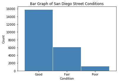
Considerably more than half of the streets are in good condition. A little less than a third are in fair condition. Only 5% are in poor condition.
# accidents injury bar graph
conditions = df['oci_desc'].value_counts()
fig = plt.figure()
conditions.plot.bar(x ='lab', y='val', rot=0, width=0.99,
                         color="steelblue")
plt.title ('Bar Graph of San Diego Street Conditions')
plt.xlabel('Condition')
plt.ylabel('Count')
plt.show()

conditions
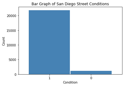
Whereas a method can be used to classify street conditions into multiple classes, it is easier to re-classify streets in “fair” and “good” condition into one category in comparison with the poor class. This, in turn, becomes a binary classification problem. Thus, there are now 21,863 streets in good condition and 1,142 in poor condition (only 5% of all streets). This presents a definitive example of class imbalance.
df['oci_cat'] = df['oci_desc'].map({'Good':1, 'Fair':1,
                                    'Poor':0})
cond = df['oci_cat'].value_counts()
cond
# oci ratings bar graph
fig = plt.figure()
cond.plot.bar(x ='lab', y='val', rot=0, width=0.99,
                         color="steelblue")
plt.title ('Bar Graph of San Diego Street Conditions')
plt.xlabel('Condition')
plt.ylabel('Count')
plt.show()

cond
# cast oci info into range of values
labels = [ "{0} - {1}".format(i, i + 5) for i in range(0, 100, 10) ]
df['OCI Range'] = pd.cut(df.oci, range(0, 105, 10),
                                right=False,
                                labels=labels).astype(object)
# inspect the new dataframe with this info
df[['oci', 'OCI Range']]
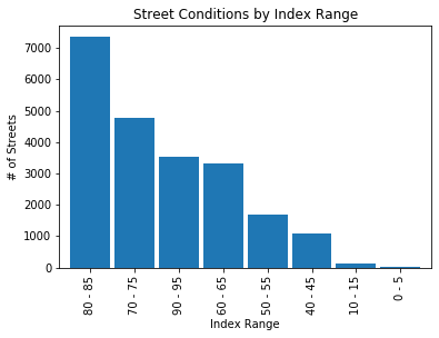
print("\033[1m"+'Street Conditions by Condition Index Range'+"\033[1m")
def oci_cond():
    oci_desc_good = df.loc[df.oci_desc == 'Good'].groupby(
                               ['OCI Range'])[['oci_desc']].count()
    oci_desc_good.rename(columns = {'oci_desc':'Good'}, inplace=True)
    oci_desc_fair = df.loc[df.oci_desc == 'Fair'].groupby(
                               ['OCI Range'])[['oci_desc']].count()
    oci_desc_fair.rename(columns = {'oci_desc':'Fair'}, inplace=True)
    oci_desc_poor = df.loc[df.oci_desc == 'Poor'].groupby(
                               ['OCI Range'])[['oci_desc']].count()
    oci_desc_poor.rename(columns = {'oci_desc':'Poor'}, inplace=True)
    oci_desc_comb = pd.concat([oci_desc_good, oci_desc_fair, oci_desc_poor],
    axis = 1)
    # sum row totals
    oci_desc_comb.loc['Total']= oci_desc_comb.sum(numeric_only=True, axis=0)
    # sum column totals
    oci_desc_comb.loc[:,'Total'] = oci_desc_comb.sum(numeric_only=True, axis=1)
    oci_desc_comb.fillna(0, inplace = True)
    return oci_desc_comb.style.format("{:,.0f}")

oci_cond = oci_cond().data # retrieve dataframe
oci_cond
oci_plt = oci_cond['Total'][0:8].sort_values(ascending=False)
oci_plt.plot(kind='bar', width=0.90)
plt.title('Street Conditions by Index Range')
plt.xlabel('Index Range')
plt.ylabel('# of Streets')
plt.show()
3.2 Summary Statistics
# summary statistics
summ_stats = pd.DataFrame(df['oci'].describe()).T
summ_stats
IQR = summ_stats['75%'][0] - summ_stats['25%'][0]
low_outlier = summ_stats['25%'][0] - 1.5*(IQR)
high_outlier = summ_stats['75%'][0] + 1.5*(IQR)
print('Low Outlier:', low_outlier)
print('High Outlier:', high_outlier)
print("\033[1m"+'Overall Condition Index (OCI) Summary'+"\033[1m")
def oci_by_range():
    pd.options.display.float_format = '{:,.2f}'.format
    new = df.groupby('OCI Range')['oci']\
    .agg(["mean", "median", "std", "min", "max"])
    new.loc['Total'] = new.sum(numeric_only=True, axis=0)
    column_rename = {'mean': 'Mean', 'median': 'Median',
                     'std': 'Standard Deviation',\
                     'min':'Minimum','max': 'Maximum'}
    dfsummary = new.rename(columns = column_rename)
    return dfsummary
oci_by_range = oci_by_range()
oci_by_range
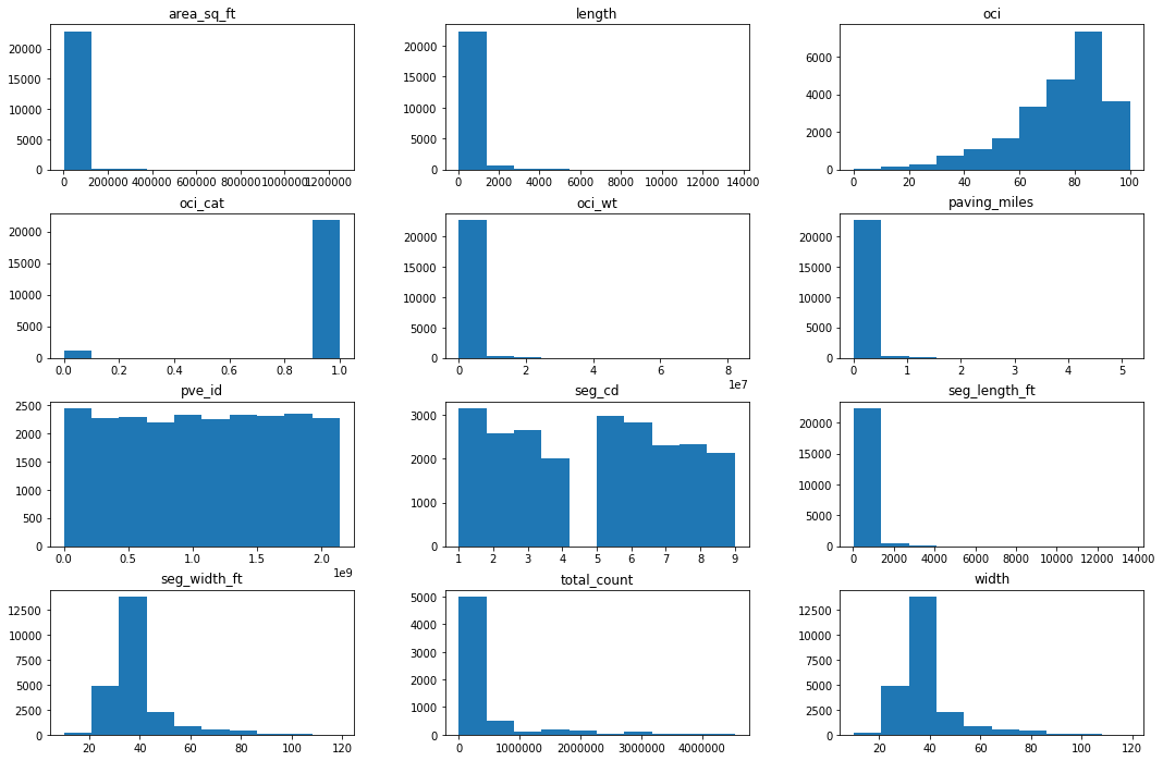
3.3 Histogram Distributions
# histograms
df.hist(grid=False, figsize=(18,12))
plt.show()
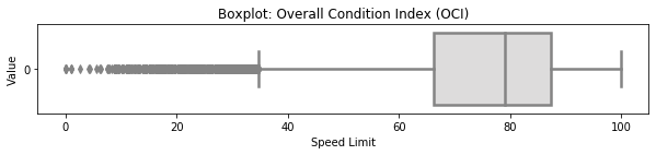
3.4 Boxplot Distribution (OCI)
# selected boxplot distribution for oci values
print("\033[1m"+'Boxplot Distribution'+"\033[1m")

# Boxplot of age as one way of showing distribution
fig = plt.figure(figsize = (10,1.5))
plt.title ('Boxplot: Overall Condition Index (OCI)')
plt.xlabel('Speed Limit')
plt.ylabel('Value')
sns.boxplot(data=df['oci'],
            palette="coolwarm", orient='h',
            linewidth=2.5)
plt.show()

IQR = summ_stats['75%'][0] - summ_stats['25%'][0]

print('The first quartile is %s. '%summ_stats['25%'][0])
print('The third quartile is %s. '%summ_stats['75%'][0])
print('The IQR is %s.'%round(IQR,2))
print('The mean is %s. '%round(summ_stats['mean'][0],2))
print('The standard deviation is %s. '%round(summ_stats['std'][0],2))
print('The median is %s. '%round(summ_stats['50%'][0],2))
3.5 Correlation Matrix
# assign correlation function to new variable
corr = df.corr()
matrix = np.triu(corr) # for triangular matrix
plt.figure(figsize=(10,10))
# parse corr variable intro triangular matrix
sns.heatmap(df.corr(method='pearson'),
            annot=True, linewidths=.5,
            cmap="coolwarm", mask=matrix,
            square = True,
            cbar_kws={'label': 'Correlation Index'},
            vmin=-1, vmax=1)
plt.show()
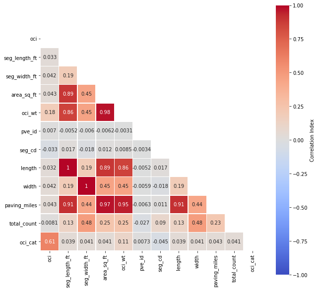
3.6 Multicollinearity
Let us narrow our focus by removing highly correlated predictors and passing the rest into a new dataframe.
cor_matrix = df.corr().abs()
upper_tri = cor_matrix.where(np.triu(np.ones(cor_matrix.shape),
                                     k=1).astype(np.bool))

to_drop = [column for column in upper_tri.columns if
           any(upper_tri[column] > 0.75)]
print('These are the columns prescribed to be dropped: %s'%to_drop)
4 Pre-Processing
Based on the prescribed output of the multicollinearity outcome, we should remove area_sq_ft, oci_wt, length, width, paving_miles, respectively. However, area in square feet is derived from length (x) width values, and converted to paving miles. Removing all of these features is not necessary. We can keep area in square feet, as long as we remove the rest.
4.1 Feature Engineering
The start date is subtracted from the end date and converted to number of days as one column.
df['date_end'] = pd.to_datetime(df['date_end'])
df['date_start'] = pd.to_datetime(df['date_start'])
# 7 rows with missing values are dropped in the following line
day_diff = df.dropna(subset=['date_end', 'date_start'],inplace=True)
df['day_diff'] = (df['date_end'] - df['date_start']).dt.days.astype(int)
zero_days = df['day_diff'].value_counts()[0]
percent_days = round(zero_days/len(df), 2)*100
print('There are', zero_days, 'rows with "0".')
print('That is roughly', percent_days, '% of the data.')
The residential, collector, major, prime, local, and alley functional classes are converted to dummy variables.
df['func_class'].value_counts()
df['func_cat'] = df['func_class'].map({'Residential': 1,
                                       'Collector': 2,
                                       'Major': 3, 'Prime':4,
                                       'Local':5, 'Alley':6})
The AC Improved, PCC Jointed Concrete, AC Unimproved, and UnSurfaced pavement classes are converted to dummy variables.
df['pvm_class'].value_counts()
df['pvm_cat'] = df['pvm_class'].map({'AC Improved': 1,
                                     'PCC Jointed Concrete': 2,
                                     'AC Unimproved': 3,
                                     'UnSurfaced':4})
The current status of the job (i.e., post construction, design, bid/award, construction, and planning) is also converted to dummy variables.
df['status'].value_counts()
df['status_cat'] = df['status'].map({'post construction': 1,
                                     'design': 2,
                                     'bid / award': 3,
                                     'construction':4,
                                     'planning': 5})
4.2 Dropping Non-Useful/Re-classed Columns
Columns with explicit titles (i.e., names) and non-convertible/non-meaningful strings are dropped. Redundant columns (columns that have been cast to dummy variables) have also been dropped in conjunction with the index column which serves no purpose for this experiment.
# drop unnecessary columns

df = df.drop(columns=['street_from','street_to',
                      'street_name','seg_id', 'street',
                      'pve_id', 'title','project_manager',
                      'project_manager_phone', 'project_id',
                      'resident_engineer', 'address_street',
                      'date_moratorium', 'OCI Range', 'total_count'])

df = df.reset_index(drop=True)

# drop variables exhibiting multicollinearity
df = df.drop(columns=['seg_length_ft', 'seg_width_ft',
                      'length', 'width', 'paving_miles',
                      'oci_wt'])

# drop re-classed columns
df = df.drop(columns=['func_class', 'pvm_class', 'status',
                      'type','date_end', 'date_start',
                      'oci_desc'])
The original dataframe is copied into a new dataframe df1 in order to continue the final steps in the preprocessing endeavor. This is to avoid any mis-steps or adverse/unintended effects on the original dataframe.
# create new dataframe for final pre-processing steps
df1 = df.copy()
One consequence of pre-processing data is that additional missing values may be brought into the mix, so one final sanity check for this phenomenom is commenced as follows.
df_check = df.isna().sum()
df_check[df_check>0]
cor_matrix = df.corr().abs()
upper_tri = cor_matrix.where(np.triu(np.ones(cor_matrix.shape),
                                     k=1).astype(np.bool))

to_drop = [column for column in upper_tri.columns if
           any(upper_tri[column] > 0.75)]
print('These are the columns prescribed to be dropped: %s'%to_drop)
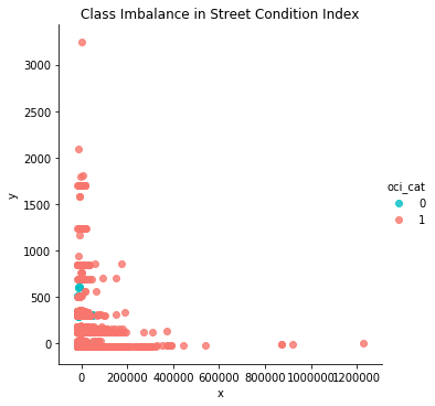
4.3 Handling Class Imbalance
Multiple methods for balancing a dataset exist like “undersampling the majority classes” (Fregly & Barth, 2021, p. 178). To account for the large gap (95%) of mis-classed data on the “poor” condition class, “oversampling the minority class up to the majority class” (p. 179) is commenced. However, such endeavor cannot proceed in good faith without the unsupervised dimensionality reduction technique of Principal Component Analysis (PCA), which is carried out “to compact the dataset and eliminate irrelevant Features” (Naseriparsa & Kashani, 2014, p. 33). In this case, a new dataframe is reduced down into the first two principal components since the largest percent variance explained exists therein.
# the first two principal components are used
pca = PCA(n_components=2, random_state=777)
data_2d = pd.DataFrame(pca.fit_transform(df1.iloc[:,0:9]))
The dataframe is prepared for scatterplot analysis as follows.
data_2d = pd.concat([data_2d, df1['oci_cat']], axis=1)
data_2d.columns = ['x', 'y', 'oci_cat']; data_2d
sns.lmplot('x','y', data_2d, fit_reg=False, hue='oci_cat',
                    palette=['#00BFC4', '#F8766D'])
plt.title('Class Imbalance in Street Condition Index'); plt.show()
The dataset is oversampled into a new dataframe df2.
The adaptive synthetic sampling approach (ADAYSN) is leveraged “where more synthetic data is generated for minority class examples that are harder to learn compared to those minority examples that are easier to learn” (He et al., 2008). This allows for the minority class to be more closely matched (up-sampled) to the majority class for an approximately even 50/50 weight distribution.
ada = ADASYN(random_state=777)
X_resampled, y_resampled = ada.fit_resample(df1.iloc[:,0:7],
                                            df1['oci_cat'])
df2 = pd.concat([pd.DataFrame(X_resampled),
                 pd.DataFrame(y_resampled)], axis=1)
df2.columns = df1.columns
The classes are re-balanced in a new dataframe using oversampling:
# rebalanced classes in new df
df2['oci_cat'].value_counts()
zero_count = df2['oci_cat'].value_counts()[0]
one_count = df2['oci_cat'].value_counts()[1]
zero_plus_one = zero_count + one_count

print('Poor Condition Size:', zero_count)
print('Good Condition Size:', one_count)
print('Total Condition Size:', zero_plus_one)
print('Percent in Poor Condition:', round(zero_count/zero_plus_one,2))
print('Percent in Good Condition:', round(one_count/zero_plus_one,2))
The dataframe can now be prepared as a flat .csv file if so desired.
4.4 Train-Test-Validation Split
#Divide train set by .7, test set by .15, and valid set .15
size_train = 30500
size_valid = 6536
size_test = 6536
size_total = size_test + size_valid + size_train
train, test = train_test_split(df2, train_size = size_train,\
                               random_state = 777)
valid, test = train_test_split(test, train_size = size_valid,\
                               random_state = 777)

print('Training size:', size_train)
print('Validation size:', size_valid)
print('Test size:', size_test)
print('Total size:', size_train + size_valid + size_test)
print('Training percentage:', round(size_train/(size_total),2))
print('Validation percentage:', round(size_valid/(size_total),2))
print('Test percentage:', round(size_test/(size_total),2))
# define (list) the features
X_var = list(df2.columns)

# define the target
target ='oci_cat'
X_var.remove(target)
X_train = train[X_var]
y_train = train[target]
X_test = test[X_var]
y_test = test[target]
X_valid = valid[X_var]
y_valid = valid[target]
# rearrange columns so that the target column is set up first
# for later training
df2 = df2[['oci_cat', 'oci', 'area_sq_ft', 'seg_cd', 'day_diff',
           'func_cat', 'pvm_cat', 'status_cat']]
# reinspect the dataframe
df2.head()
4.5 Transfer The Final Dataframe (df2) to S3 Bucket
s3_client = boto3.client("s3")
BUCKET='waterteam1'
KEY='raw_files/df2/df2.csv'
response = s3_client.get_object(Bucket=BUCKET, Key=KEY)

with io.StringIO() as csv_buffer:
    df2.to_csv(csv_buffer, index=False, header=True)

    response = s3_client.put_object(
        Bucket=BUCKET, Key=KEY, Body=csv_buffer.getvalue()
    )
5 Modeling and Training
5.1 Logistic Regression
Herein, the classical Anaconda-based scikit-learn approach is leveraged to train the logistic regression model on the validation set.
# Un-Tuned Logistic Regression Model
logit_reg = LogisticRegression(random_state=777)
logit_reg.fit(X_train, y_train)

# Predict on validation set
logit_reg_pred1 = logit_reg.predict(X_valid)

# accuracy and classification report (Untuned Model)
print('Untuned Logistic Regression Model')
print('Accuracy Score')
print(accuracy_score(y_valid, logit_reg_pred1))
print('Classification Report \n',
       classification_report(y_valid, logit_reg_pred1))
Next, the logistic regression model is tuned using RandomizedSearchCV() and cross validated using repeated stratified kfold with five splits and two repeats. A set of hyperparamaters are subsequently defined to produce an overall best accuracy score in conjunction with a set of optimal hyperparameters.
model1 = LogisticRegression(random_state=777)
cv = RepeatedStratifiedKFold(n_splits=5, n_repeats=2,
                             random_state=777)
space = dict()

# define search space
space['solver'] = ['newton-cg', 'lbfgs', 'liblinear']
space['penalty'] = ['none', 'l1', 'l2', 'elasticnet']
space['C'] = loguniform(1e-5, 100)

# define search
search = RandomizedSearchCV(model1, space,
                            scoring='accuracy',
n_jobs=-1, cv=cv, random_state=777)

# execute search
result = search.fit(X_train, y_train)

# summarize result
print('Best Score: %s' % result.best_score_)
print('Best Hyperparameters: %s' % result.best_params_)
6 Training, Testing, and Deploying a Model with Amazon SageMaker's Built-in XGBoost Model
# Define IAM role
role = get_execution_role()

# set the region of the instance
my_region = boto3.session.Session().region_name

# this line automatically looks for the XGBoost image URI and
# builds an XGBoost container.
xgboost_container = sagemaker.image_uris.retrieve("xgboost",
                                                  my_region,
                                                  "latest")

print("Success - the MySageMakerInstance is in the " + my_region + \
      " region. You will use the " + xgboost_container + \
      " container for your SageMaker endpoint.")
train, test = np.split(df2.sample(frac=1, random_state=777),
                                 [int(0.7 * len(df2))])
print(train.shape, test.shape)
6.1 Transfer The Training Data to S3 Bucket
s3_client = boto3.client("s3")
BUCKET='waterteam1'
KEY='raw_files/train/train.csv'
response = s3_client.get_object(Bucket=BUCKET, Key=KEY)

with io.StringIO() as csv_buffer:
    train.to_csv(csv_buffer, index=False, header=False)

    response = s3_client.put_object(
        Bucket=BUCKET, Key=KEY, Body=csv_buffer.getvalue()
    )
# input training parameters
s3_input_train = sagemaker.inputs.TrainingInput(s3_data=\
        's3://{}/raw_files/train'.format(BUCKET), content_type='csv')
6.2 Setting up the SageMaker Session and Supplying Instance for XGBoost Model
sess = sagemaker.Session()
xgb = sagemaker.estimator.Estimator(xgboost_container,role,
                                    instance_count=1,
                                    instance_type='ml.m5.large',
                                    output_path='s3://{}/output'.format(BUCKET),
                                    sagemaker_session=sess)
# parse in the hyperparameters
xgb.set_hyperparameters(max_depth=5,eta=0.2,gamma=4,min_child_weight=6,
                        subsample=0.8,silent=0,
                        objective='binary:logistic',num_round=100)
6.3 Train The Model
xgb.fit({'train': s3_input_train})
6.4 Deploying The Predictor
xgb_predictor = xgb.deploy(initial_instance_count=1,
                           instance_type='ml.m5.large')
6.5 Running Predictions
from sagemaker.serializers import CSVSerializer

# load the data into an array
test_array = test.drop(['oci_cat'], axis=1).values

# set the serializer type
xgb_predictor.serializer = CSVSerializer()

# predict!
predictions = xgb_predictor.predict(test_array).decode('utf-8')

# and turn the prediction into an array
predictions_array = np.fromstring(predictions[1:], sep=',')
print(predictions_array.shape)
6.6 Evaluating The Model
cm = pd.crosstab(index=test['oci_cat'],
                 columns=np.round(predictions_array),
                 rownames=['Observed'],
                 colnames=['Predicted'])
tn = cm.iloc[0,0]; fn = cm.iloc[1,0]; tp = cm.iloc[1,1];
fp = cm.iloc[0,1]; p = (tp+tn)/(tp+tn+fp+fn)*100
print("\n{0:<20}{1:<4.1f}%\n".format("Overall Classification Rate: ", p))
print("{0:<15}{1:<15}{2:>8}".format("Predicted", "Poor Condition",
                                    "Good Condition"))
print("Observed")
print("{0:<15}{1:<2.0f}% ({2:<}){3:>6.0f}% ({4:<})".format("Poor Condition", \
                                        tn/(tn+fn)*100,tn, fp/(tp+fp)*100, fp))
print("{0:<16}{1:<1.0f}% ({2:<}){3:>7.0f}% ({4:<}) \n".format("Good Condition", \
                                        fn/(tn+fn)*100,fn, tp/(tp+fp)*100, tp))
6.7 Terminating the Endpoint To Save on Costs
# clean-up by deleteting endpoint
xgb_predictor.delete_endpoint(delete_endpoint_config=True)
References
Amazon Web Services. (n.d.). Amazon Athena.
https://aws.amazon.com/athena/?whats-new-cards.sort-by=item.additionalFields.postDateTime&whats-new-cards.sort-order=desc
Amazon Web Services. (n.d.). Build, train, and deploy a machine learning model with Amazon SageMaker.
https://aws.amazon.com/getting-started/hands-on/build-train-deploy-machine-learning-model-sagemaker/
Fregly, C., & Barth, A. (2021). Data Science on AWS. O'Reilly.
Garrick, D. (2021, September 12). San Diego to spend $700K assessing street conditions to spend repair
money wisely. The San Diego Union-Tribune.
https://www.sandiegouniontribune.com/news/politics/story/2021-09-12/san-diego-to-spend-700k-assessing-street-conditions-to-spend-repair-money-wisely
He, H., Bai, Y., Garcia, E. & Li, S. (2008). ADASYN: Adaptive synthetic sampling approach for imbalanced
learning.
2008 IEEE International Joint Conference on Neural Networks (IEEE World Congress
on Computational Intelligence),1322-1328.
https://ieeexplore.ieee.org/document/4633969
Naseriparsa, M. & Kashani, M.M.R. (2014). Combination of PCA with SMOTE Resampling to Boost the Prediction Rate in Lung Cancer Dataset.
International Journal of Computer Applications, 77(3) 33-38. https://doi.org/10.5120/13376-0987